score centering

I'm surprised at how persistent of a problem the train-inference mismatch (TIM) has turned out to be. If memory serves me it was first raised in one of the MiniMax reports back in spring 2025, ~18 months later we're still here talking about it.

TIM approaches have generally fallen into two camps: (1) accept the mismatch and correct for it, usually folding in staleness and other sources of off-policyness along the way: TIS, MIS, IcePop, DPPO, and friends (2) explicitly reduce or even eliminate the mismatch. At the heavy end that means unifying the training and inference stacks (shared kernels, batch invariance). Lighter fixes include an FP32 LM head, BF16 across train and rollout, router replay etc. Frontier open labs have made different bets along these two axes. I figured we would have converged on a solution by now, perhaps todays topic will edge is closer to that reality :)

We study score centering, an orthogonal and complementary approach to addressing TIM. I'm not if there's a research lineage here or if this paper kind of came out of the blue, but everything today comes from reading Score Centering Stabilizes Off-policy Reinforcement Learning.

we begin with the policy gradient

Consider the simplest possible objective:

$$\mathcal{J}(\theta)=\mathbb{E}_{a\sim p_\theta}[R(a)]$$

This denotes the expected reward as we sample actions from our policy $p_\theta$. For simplicity, we'll consider a single next-token decision at a fixed prefix, leaving the prefix implicit in our notation.

We want to know how to update our parameters $\theta$ such as to maximize this objective. The problem is that $\theta$ doesn't appear directly inside the reward function. Instead, it determines the distribution from which we sample our actions. Through some mathematical tricks we can derive the typical policy gradient. See Nathan Lambert's RLHF book for more details.

$$\nabla_\theta\mathcal{J}(\theta) =\mathbb{E}_{a\sim p_\theta} \left[ R(a)\nabla_\theta\log p_\theta(a) \right]$$

Note here that the reward does not need to be differentiable. Importantly, the second factor in the expression is known as the score function:

$$\boxed{ s_\theta(a)=\nabla_\theta\log p_\theta(a) }$$

This has nothing to do with the reward score. Rather, the score represents the gradient w.r.t. the model parameters of the log-probability of the sampled action.

When denoted this way, we see that the core structure of the policy gradient is really just the reward multiplied by the score:

$$\nabla_\theta\mathcal{J}(\theta) = \mathbb{E}_{a\sim p_\theta} \left[ R(a)s_\theta(a) \right]$$

The reward tells us whether the action should be reinforced or weakened and by how much, while the score tells us which direction the parameters need to move in to raise or lower the probability of said action. Note that all of this comes down to the score, the gradient of the action log-probability.

the score function identity

The score function has an interesting property: its expectation under its own distribution is zero

$$\boxed{ \mathbb{E}_{a\sim p_\theta}[s_\theta(a)]=0 }$$

known as the score function identity, which we can prove directly

$$\begin{aligned} \mathbb{E}_{a\sim p_\theta}[s_\theta(a)] &=\sum_a p_\theta(a)\nabla_\theta\log p_\theta(a)\\ &=\sum_a\nabla_\theta p_\theta(a)\\ &=\nabla_\theta\sum_a p_\theta(a)\\ &=\nabla_\theta 1\\ &=0 \end{aligned}$$

Simple enough, but I think it's useful to look at the score in more detail to understand why this happens and, more importantly, what happens when we go off-policy. Recall that the output probabilities are produced by applying softmax to the model's logits, the probability action $a$ is hence:

$$p_\theta(a)=\frac{e^{z_a}}{\sum_j e^{z_j}}$$

Taking the log:

$$\log p_\theta(a)=z_a-\log\sum_j e^{z_j}$$

and differentiating with respect to one logit $z_i$:

$$\frac{\partial\log p_\theta(a)}{\partial z_i} = \underbrace{\frac{\partial z_a}{\partial z_i}}_{\mathbf{1}[i=a]} - \underbrace{ \frac{\partial}{\partial z_i} \log\sum_j e^{z_j} }_{p_\theta(i)}$$

The second term is simply the softmax probability of token $i$, since

$$\frac{\partial}{\partial z_i} \log\sum_j e^{z_j} = \frac{e^{z_i}}{\sum_j e^{z_j}} = p_\theta(i)$$

Therefore:

$$\boxed{ \frac{\partial\log p_\theta(a)}{\partial z_i} = \mathbf{1}[i=a]-p_\theta(i) }$$

Collecting the partial derivatives for every logit gives:

$$\boxed{ \nabla_z\log p_\theta(a) = \underbrace{e_a}_{\text{one-hot vector}} - \underbrace{p_\theta}_{\text{probability vector}} }$$

This provides a nice intuition: the gradient is positive for the chosen action and negative for all other actions. The magnitude of the negative gradients is proportional to their probabilities, while the gradient for the chosen action is $1-p_\theta(a)$, meaning it becomes smaller as the model becomes more confident in that action.

Now, let's substitute this expression back into the expectation over the score, still working in logit space

$$\mathbb{E}_{a\sim p_\theta} \left[ \nabla_z\log p_\theta(a) \right]$$

and substitute in our gradient expression:

$$= \mathbb{E}_{a\sim p_\theta}[e_a-p_\theta]$$

By linearity of expectation:

$$= \mathbb{E}_{a\sim p_\theta}[e_a]-p_\theta$$

We focus on $\mathbb{E}[e_a]$. Since $e_a$ is a one-hot vector, its expectation is simply the probability distribution itself:

$$\mathbb{E}_{a\sim p_\theta}[e_a] = \sum_a p_\theta(a)e_a = p_\theta \tag{A}$$

which means

$$\boxed{ \mathbb{E}_{a\sim p_\theta} \left[ \nabla_z\log p_\theta(a) \right] = p_\theta-p_\theta=0 }$$

arriving back at the zero mean property. Importantly notice that this outcome is dependent on the assumption that actions were sampled from the same distribution used to compute the score, otherwise (A) doesn't equal $p_\theta$.

what happens under train-inference mismatch?

In practice, our rollouts aren't necessarily sampled from the current trainer distribution $p_\theta$. Instead, they're generated by a separate inference engine, whose distribution we'll denote $q_\varphi$. The two distributions can differ because of numerical differences between training and inference, quantization, or simply because the generator is running an older version of the trainer. Consequently, we're sampling actions from $q_\varphi$, while computing their score under $p_\theta$.

Let's revisit the expectation of the score under these conditions. Previously, we established that the gradient of the log-probability w.r.t. the logits is $e_a-p_\theta$. However, if our actions are sampled from $q_\varphi$, the expectation becomes

$$\begin{aligned} \mathbb{E}_{a\sim q_\varphi} \left[ \nabla_z\log p_\theta(a) \right] &= \mathbb{E}_{a\sim q_\varphi} [e_a-p_\theta]\\ &= q_\varphi-p_\theta \end{aligned}$$

Suddenly

$$\boxed{ \mathbb{E}_{a\sim q_\varphi} \left[ \nabla_z\log p_\theta(a) \right] = q_\varphi-p_\theta\neq 0 }$$

we've broken the zero-mean property. The expected score is no longer zero, but instead depends on the difference between the generator and trainer distributions.

The drift term

How does this materialize inside our policy gradient?

Let $A(a)$ denote advantage from here on. Under the generator distribution, the expected update is $\mathbb{E}_{a\sim q_\varphi}[A(a)s_\theta(a)]$. Using the covariance identity, we can decompose this into two terms:

$$\boxed{ \mathbb{E}_{q_\varphi}[As_\theta] = \underbrace{ \mathbb{E}_{q_\varphi}[A]\bar{s} }_{\text{drift}} + \underbrace{ \operatorname{Cov}_{q_\varphi}(A,s_\theta) }_{\text{learning signal}} }$$

This is one of the central observations in the paper. The second term is what we're interested in. It captures the relationship between the sampled actions and their rewards, reinforcing actions with relatively higher advantages and weakening those with relatively lower advantages. The first term, however, is problematic. The drift term carries no information about which actions were successful. It depends on the advantages only through their mean, $\mathbb{E}_{q_\varphi}[A]$, meaning it can produce an update even without any relationship between which action was sampled and how well it performed. It turns out in fact that the first term acts as a distillation objective towards the sampler, scaled by the expected reward. On-policy this has no effect, the trainer already matches the sample, so $\bar s = 0$ (also score identify function) and hence the drift term vanishes completely. Distillation toward a fixed teacher is harmless, the sampler however is not fixed, in RL its a biased copy of the trainer (quantization, stale, numerically mismatched, ...) so what happens is that each step pushes the trainer toward the sampler.

As we've established, under TIM this drift term is non-zero because $\bar s = \mathbb{E}_{q_\varphi}[s] \neq 0$. Consequently you end up with a gradient despite there clearly being any learning signal in the rollouts. Take for example the extreme case $R = 1$ for every action. This gives

$$\operatorname{Cov}_{q_\varphi}(A,s_\theta) = 0$$

but the policy gradient

$$\boxed{ \mathbb{E}_{q_\varphi}[As_\theta] = \bar{s} } \neq 0$$

which means we're now updating our model despite having received absolutely no information about which actions are preferable. And as we said earlier the direction of this update turns out to effectively be a distillation gradient toward the sampler. We can derive this formally quickly, what we are interested in is the direction of $\bar s$. Remember that

$$\bar{s} = \mathbb{E}_{a\sim q_\varphi} [\nabla_\theta\log p_\theta(a)]$$

This is actually the negative gradient of the cross-entropy loss when treating the generator as the teacher:

$$\boxed{ \bar{s} = -\nabla_\theta H(q_\varphi,p_\theta) }$$

where

$$H(q_\varphi,p_\theta) = -\sum_a q_\varphi(a)\log p_\theta(a)$$

so we end up with this completely uniformative signal, when mean advantage is positive the drift term distills toward the generator, and when its negative it pushes away from the generator. Clearly neither direction is influenced by which individual actions produce better rewards...

This term is an artifact of TIM

Score centering

With the drift term identified, score centering actually becomes very intuitive. We want to restore the zero-mean property of the score under the distribution that generated our actions. The whole problem comes from sampling actions from $q_\varphi$ while using $p_\theta$ to center the score, so instead of centering with the trainer distribution, we center with the generator distribution. In other words, remove the drift term! Recall the score function of the training policy $p_\theta$:

$$s_\theta(a)=\nabla_\theta \log p_\theta(a)$$

Using the covariance identity, we've shown that the policy gradient can be expressed as:

$$\boxed{ \mathbb{E}_{q_\varphi}[As_\theta] = \underbrace{ \mathbb{E}_{q_\varphi}[A]\bar{s} }_{\text{drift}} + \underbrace{ \operatorname{Cov}_{q_\varphi}(A,s_\theta) }_{\text{learning signal}} }$$

Under TIM we sample from $q$ while computing scores through $p$. Consequently:

$$\mathbb{E}_q[s]\neq 0$$

Our goal is to ensure the expected score is zero, even when $q\neq p$. We achieve this by defining a new, centered score function:

$$\boxed{ \tilde{s}_\theta(a) = s_\theta(a)-\mathbb{E}_q[s_\theta] }$$

Replacing the old score with the centered score in our policy gradient objective from equation 3

$$\begin{aligned} \mathbb{E}_q[R\tilde{s}] &= \mathbb{E}_q[R(s-\mathbb{E}_q[s])] \\[6pt] &= \mathbb{E}_q[Rs]-\mathbb{E}_q[R]\mathbb{E}_q[s] \\[6pt] &= \underbrace{\operatorname{Cov}_q(R,s)}_{\text{signal}} +\underbrace{\mathbb{E}_q[R]\mathbb{E}_q[s]}_{\text{drift}} -\underbrace{\mathbb{E}_q[R]\mathbb{E}_q[s]}_{\text{centering correction}} \\[6pt] &= \operatorname{Cov}_q(R,s) \end{aligned}$$

leaving us with only the learning signal!

practical implementation

Normally, during training, we perform a forward pass through the trainer, compute the log-probabilities using log-softmax, and construct our policy gradient loss. But as we've seen, differentiating through the standard log-softmax necessarily produces the gradient $e_a-p_\theta$. We cannot get our desired gradient $e_a-q_\varphi$ by simply computing the usual log-probability loss, so we need to modify the objective.

The paper proposes expressing score centering as a scalar loss:

$$\boxed{ \mathcal{L}_{\mathrm{SC}} = -A(a) \left[ \log p_\theta(a) - \sum_v \operatorname{sg}[q_\varphi(v)] \log p_\theta(v) \right] }$$

Here, $\operatorname{sg}$ denotes stop-gradient. The log-probabilities $\log p_\theta$ still come from the current trainer's forward pass, while the generator probabilities $q_\varphi$ are used only to weight the centering term. We don't differentiate through the generator probabilities, and the advantage is also treated as fixed. Differentiating the loss w.r.t. the trainer's logits gives

$$\boxed{ \nabla_{z_\theta}\mathcal{L}_{\mathrm{SC}} = -A(a)(e_a-q_\varphi) }$$

which is exactly what we want! Notice that we're still computing gradients through the current trainer, but have modified the loss such that the resulting gradient is centered using the generator's distribution instead of the trainer's.

Okay, but what does this require in practice? Looking at the loss, the second term requires the generator's probability distribution over the entire vocabulary at every generated token position. This is highly infeasible, particularly when generating long rollouts across large batches. Storing and communicating vocabulary-sized probability vectors between the generator and trainer would introduce substantial memory and communication overhead.

Instead, the authors propose an approximation where they store only the generator's top-$k$ log-probabilities and approximate the remaining probability mass using the trainer's distribution, rescaled to match the generator's tail mass. This allows them to compute an approximate centering correction using only a small subset of the vocabulary. In their experiments, they use $k=128$ and find that even $k=32$ performs comparably to full score centering across their tested settings. This is just one of the many possible ways of approximating the generators distribution, the experiment results suggest its a viable one.

Importance sampling + score centering

Great, we've centered the score properly. So what does this mean w.r.t. importance sampling? Can we just skip that entirely now that the score is centered?

Not quite. These are separate issues. We've restored the zero-mean property, but we are still learning under the generator distribution; after score centering, our expected update in logit space is

$$\boxed{ g_{\mathrm{SC}} = \mathbb{E}_{a\sim q_\varphi} [A(a)(e_a-q_\varphi)] = \operatorname{Cov}_{q_\varphi}(A,e_a) }$$

We've removed the drift term that depended only on the mean advantage, leaving us with the covariance between the advantage and the sampled action. But importantly, this covariance is still measured under $q_\varphi$! The current trainer's on-policy gradient would instead be

$$\boxed{ g_p = \mathbb{E}_{a\sim p_\theta} [A(a)(e_a-p_\theta)] = \operatorname{Cov}_{p_\theta}(A,e_a) }$$

This is the remaining problem that importance sampling addresses. While score centering removes the unwanted drift, importance sampling attempts to correct the distribution mismatch by reweighting samples according to how likely they would have been under the current trainer. In theory, exact importance sampling recovers the on-policy expectation, but in practice these ratios can be very large so they are typically clipped or masked, which takes us back to TIS/MIS/DPPO variants.

---

Under severe quantization-induced TIM, score centering alone performs particularly well, often outperforming importance-sampling-based corrections. Under heavy staleness, however, combining score centering with TIS or MIS performs better than score centering alone. This is consistent with our earlier observation: score centering removes the drift, but the remaining covariance is still measured under the generator. When the generator becomes sufficiently stale, correcting that distribution mismatch becomes increasingly important.

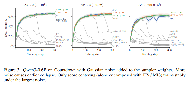
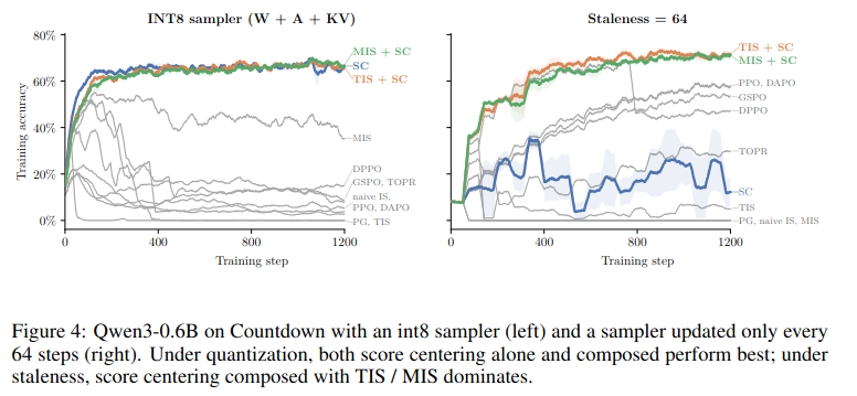
worth noting that the experiments are somewhat synthetic by nature where the authors deliberately amplify TIM rather than relying on its natural occurrence, as that typically requires long training runs.