GLM 5.3 Flash (26 Aug)

GLM drops a Flash variant of the 5 series. This is the first flash model since 4.7 Flash. The model is 320B A18B.

GLM 5 series models have all been MLA+DSA, same setup as DeepSeek V3.2, but with the addition of IndexShare since GLM 5.2. IndexShare reduces the computational cost (FLOPs) of the sparse attention mechanism by avoiding running the lightning indexer on every layer, instead top-k indexes are shared across 4 layers, so there is only one lightning indexer for every 4 layers.

GLM 5.3 Flash is the first time GLM moves to a linear attention variant. The model employs hybrid attention, alternating between linear and sparse attention: KDA and DSA(MLA) in a 3:1 ratio. This is definitely to target KV cache memory. At 128k context, GLM 5.3 requires ~12.5GB of kv cache memory, while GLM 5.3 Flash only uses 1.7GB (obv Flash is a smaller model but this reduction is far greater than just that).

With GLM dropping a linear attention variant this means all frontier chinese labs except for DeepSeek seem to be switching to linear attention. DS is yet to release a single model with linear attention, it just keeps hammering on compressed attention variants combined with sparse attention.

Qwen 3.8 (14 Aug)

Qwen 3.8 builds on the same architectural foundation as is introduced by Qwen 3.5: Hybrid attention alternating between Gated DeltaNed and Gated GQA in a 3:1 ratio.

There is a 2.4T A95B MoE variant and a 27B Dense variant.

Since switching to 3:1 GDN:GQA setup back in Qwen 80B Next last year, Qwen hasn't switched up their architecture. They've been pretty quiet on that front especially when compared to Kimi, GLM, DeepSeek. Nonetheless the popularity of Qwen's models continue, they are the defacto standard model creator in the local llm space, and they are the only chinese lab releasing models in the small-medium size range. Also the only chinese lab dropping dense models still.

Qwen 3.8 2.4T provides a very nice comparison point to Kimi K3. Both use a 3:1 linear attention to dense attention setup, with Kimi running KDA and Qwen GDN (note that KDA is very similar to GDN) and Kimi with MLA while Qwen runs Gated GQA. Kimi running MLA means their KV cache footprint is quite a lot smaller than Qwen. At 128k context K3 uses 4GB while Qwen 3.8 uses 13GB.

All hybrid attention variants we see in frontier models have converged on a 3:1 linear:global setup. The global attention choice differs, some archs have a dense attention while others employ something sparse, but either way its a global variant allowing attention between any past token position.

Qwen 3.8 Flash Next (27 Aug)

The same way Qwen3-Next laid the groundwork for the future Qwen series with hybrid GDN + Gated Attention design, Qwen 3.8 Flash Next is released to foreshadow the architecture of the upcoming Qwen 4 series.

The overall architecture while new for Qwen, is very reminiscent of the direction we've been moving in during 2026. This model upgrades the architecture across four modules - attention, residual, embedding and optimization. Let's look at them individually:

Attention 3:1 Gated DeltaNet:Qwen Sparse Attention. So that means a 3:1 linear:sparse attention setup, the same design as GLM 5.3 Flash. This sticks to the 3:1 linear:global design we've seen a lot. While GLM uses DSA, Qwen introduce their own sparse attention variant QSA.

For the linear attention layers they stick with the tried and tested GDN.

For global attention they now switch from dense GQA to a sparse QSA. QSA is an evolution of DSA, but with the goal of reducing FLOPs of the indexer "as the context grows, the indexer itself becomes a non-negligible source of computation". They reduce the job performed by the indexer by compressing keys along the sequence dimension into blocks, and have the indexer query across blocks instead of individual tokens. The top-k blocks are expanded before provided to the core attention module, so the core attention still operates on a token level representation. So at the high level: $\text{DSA: } L \xrightarrow{\text{indexer}} k$ $\text{QSA: } L \rightarrow L/r \xrightarrow{\text{indexer}} \text{selected blocks}.$ The key difference from DeepSeek CSA is what gets compressed because under CSA both the retrieval representation and the actual information being retrieved are compressed:

Both the retrieval representation and the actual information being retrieved are compressed:

$\text{main KV}: L\rightarrow L/m$ $\text{indexer K}: L\rightarrow L/m.$

The indexer selects compressed KV summaries, and CoreAttn attends directly to those summaries. While QSA compressed the indexer/search space, reducing FLOPs of the indexer. So QSA is closer to something lika DSA + block compressed indexer. Obviously the core attn still applies to the sparse result of the indexer. CSA has the gained advantage of also reducing KV cache memory.

Residuals Inspired by Hyper Connections but slightly different, termed Gated Residuals.

Gated Residuals expands the residual stream into multiple channels, same as HC does. HC has three mappings around the residual stream: residual, read, write. GR removes the residual mapping. HC implements the read mapping as a input dependent scalar

$x_l = \sum_i a_{l,i}h_l^i$ where $a_{l,i}$ is one scalar per stream. Qwen makes this considerably more fine-grained, producing a gate for every feature of every stream

$\boxed{ x_l=\frac14\sum_{i=1}^4 g_l^i\odot \operatorname{RMSNorm}(h_l^i) }$ where $g_l^i\in(0,1)^d$. So every feature dimension gets a gate and is summed together. So instead of

"read 70% of stream 1 and 20% of stream 2",

GR enables

"for these feature dimensions read stream 1, for these dimensions read stream 3, etc."

The gates are computed through a low rank MLP looking at all n residual streams together. So interestingly GR produces the gates by conditioning on all residual streams, HC operates independantly across streams. So for example under GR feature 100 of stream 1 can depend on the content of streams 2-4 as well. Qwen explicitly found predicting from all branches better than using one branch or pooling them first.

Writing back to residual stream is done with four scalar write gates

$\boxed{ h_{l+1}^i=h_l^i+s_l^i y_l. }$

so very simple. So all of Qwen's sophistication is concentrated our the read operation:

$\text{n persistent streams} \xrightarrow{\text{elementwise dynamic read}} x_l \xrightarrow{F_l} y_l \xrightarrow{\text{n scalar write strengths}} \text{n persistent streams}.$

GR applies a "Gated" style operation on the residual streams, then combines the content dependant rescaled features via fixed averagining across streams.

Qwen turns the residual state into four persistent memory lanes. Each layer can very selectively read features from those lanes and decide how strongly to write its new result into each lane, but it doesn't directly remix/rewrite the old lane contents.

Embeddings

Qwen adopts n-gram embeddings table.

n-gram tables is an embedding table that provides a learned embedding for n-grams that are injected into the hidden latent at token positions. For example consider the sequence

$[\ldots,x_{t-2},x_{t-1},x_t]$ then we can form suffix n-grams such as $(x_{t-1},x_t),\qquad (x_{t-2},x_{t-1},x_t).$ Which are hashed into a large embedding table. What's the motivation/gain here? Well this provides a mechanism for knowledge retrieval, it gives a way for the model to store information related to these n-grams without having to spend a lot of FLOPs retrieving this knowledge from for example its FFN layers (which is what we believe normally happens). Instead of having to spend these FLOPs the model can learn to store static, context independant (meaning unrelated to context outside of the n-gram) information related to n-grams. For example consider the n-gram Barack Obama, this name implicitly carries a lot of information / knowledge which a normal model has to retrieve through FFNs, but could instead store in its embedding table and retrieve. The n-gram table doesn't depend on the hidden state, so the entries can be prefetched immediately upon having the token ids, this means the tables can be offloaded to a lower memory tier and dont have to sit and consume expensive HBM. Also since we only extract a few entries from the table the memory movement is cheap.

So we know we want a lookup table for n-grams, how do we build this n-gram table? The naive approach would construct a table for every possible n-gram, but we can immediately see that this is infeasible. At a vocab size V = 200, a literal bigram table would require:

$V^2 = 40 \text{ billion}$ distinct entries, and trigrams are obviously hopeless. So instead of doing this you choose a fixed size table $E\in\mathbb R^{M\times d},$ where M is determined by the memory budget you can afford. Then for an arbitrary n-gram you compute a deterministic hash

$g=(x_{t-1},x_t),$ $j = h(g)\bmod M$

and retrieve with j into the embedding table. Naturally the price you pay here is collisions since you've got mod M you are going to end up with collisions. M controls the memory/collision trade-off. The reason this works in practice is that n-grams are far from equally likely. If all n-grams were equally likely the collisions would be disastrous, but in reality the distribution over n-grams is extremely long-tailed. The actual access distribution over n-grams is extremely skewed: a relatively small set of common phrases/patterns accounts for a large fraction of occurrences, while there is a huge tail of n-grams seen rarely. DeepSeek explicitly points out that natural-language n-grams follow a Zipfian distribution.

The natural consequence of this setup is that the embedding entry will be trained proportionally to the commonality of all possible n-grams that have that specific hash. That means the rarer the n-gram, the less information the embedding entry carries for it. If very rare n-grams collide that likely doesnt matter too much, if a frequent n-gram collides with a rare one, the shared embedding is mostly going to be trained by the most frequent one. The costly case is if two important frequent n-grams collide.

They get around this issue by splitting the embedding table into multiple "heads". Instead of having a single table holding the entire inner dimension d $E\in\mathbb R^{M\times d},$ You have multiple embedding tables each holding a split of the inner dimension. Each embedding table has its own hashing function, so a lookup means K different hashes, indexing into K different embedding tables, and then concatenating the result to form a d-dimensional vector.

One thing to note is that the typical hashing function we've seen used doesn't exploit frequency when assigning slots. A common n-gram and a rare one both just hash uniformly. Qwen actually says they experimented with things like frequency-based partitioning of embedding slots, but did not see consistent gains over the simpler scheme.

So after hashing and finding the entries for a given n-gram you end up with a d-dimensional embedding vector $e_t$. What next? Well now you want to inject this into the hidden state representation $h_t$, but you dont want to do this unconditionally. The embedding table represents information about a given n-gram, but not all n-grams contain valuable information for the given context. Depending on the overall sequence context the stored information the n-gram table may be useless, there are also a alot of n-gram entries which just generally dont contain very usable information, like consider all the n-grams for n-grams that are not nouns, like "and this", "we have", "then this". The idea is, as we see more and more in our models now adays, that we don't want to just unconditionally inject information with a pre-determined scale, instead we prefer to give the model the ability to inject information depending on context/state, and rescale it as it wishes.

So we want to add $e_t$ to $h_t$ but in a way that depends on $h_t$, allowing the model to ask roughly "Is this static n-gram memory useful in the context we've built so far?". The way we do this is with a gating function that is quite similar to attention: we start by creating a key and value representation using our looked up n-gram embedding entry: $k_t=W_K e_t,\qquad v_t=W_V e_t.$ Then we think of the current hidden state $h_t$ to represent the query. We normalize query and keys separtely, then perform the dot product between the two, producing a compatability score:

$s_t= \frac{ \operatorname{RMSNorm}(h_t)^\top \operatorname{RMSNorm}(k_t) }{ \sqrt d }.$ Then $\boxed{\alpha_t=\sigma(s_t)\in(0,1)}$ We apply this scalar gate to the projected value vector $v_t$

$\tilde v_t=\alpha_t v_t.$ and add this result to $h_t$

$h_t = h_t + \tilde v_t$

Mimo V2.6 (21 Sep)

V2.6 Pro: 1T A42B V2.6 Flash: 310B A15B

Standard architectures. Nothing special. Multimodal: text,audio,images.

80% of the tech report is dedicated to the RL stage.

Meta Superintelligence Labs

Just want to disentangle all the model releases from MSL so that we know what we're working with. As of October, MSL now have three closed models, going from small to big: Spark 1.3, Wonder, Wonder Full. Wonder family is separate model arch and pretrain from Spark.

Wonder is about 4x more expensive than Spark 1.3. More importantly they also released Spark Open.

Spark Open is a 3:1 SWA:GQA arch with 816B parameters activating 42B. Overall arch is standard, seems to be using gated residuals.

MiMo HySparse2 (inc: MiMo V3)

HySparse2 is a design that separates prefill from decode architecturally, meaning that only part of the network needs to be run during "prefill". The role of prefill is to produce KV cache for the decode query process, so the prefill "part" of the archtiecture of HySparse2 produces the KV cache which is then bridged into the decode part of the architecture which only uses the KV cache from the prefill stage. Let's make this more explicit.

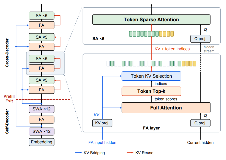
Self-Decoder and KV Bridging

We'll start by looking at the Self-Decoder. The self-decoder works like a normal SWA transformer, although with a very high SWA to global attention ratio having 12x SWA layers followed by 1 FA layer and then 12x SWA layers again. The self-decoder operates as normal, each layers QKV projections depend on the previous layer, and iteratively refine the residual stream at each token position. This is in line with conventional transformer models where each layer depends on the past.

But this is where things in HySparse2 get quirky. The model is split into

• Self-decoder: 25 layers, consisting of 24 SWA layers and one FA layer.
• Cross-decoder: 24 layers, consisting of four FA layers, each followed by five SA layers.

And once we get to the cross-encoder we are no longer computing K/V from the residual stream but rather obtaining them from earlier self-decoder layers! This is the blue path in the figure above. So

$K_j = W_j^K H_{\text{self}},\qquad V_j = W_j^V H_{\text{self}}$

So the hidden states come directly from previous self-decoder layers. Importantly however the query path is still iterative and comes from the residual stream

$Q_j = W_j^Q H_{\text{cross},j}$

This is KV Bridging.

This has a couple of implications directly. Inference pre-fill "finishes" after the first 25 layers, because at that point we've already compute the KV cache. The subsequent cross-decoder layers are only used to decode the next token prediction, so the sequence length is reduced to 1. This means prefill FLOPs are significantly reduced (only applies to half the model layers).

Note that it doesn't effect decode FLOPs, as decode still has to pass through the entire model, both decoders.

It reduces KV cache memory slightly.

KV Reuse

Now, to further improve efficiency HySparse 2 employs sharing KV within the cross decoder. Look at the RHS of the figure above, each cross-decoder block contains:

FA → SA → SA → SA → SA → SA

The FA layer receives the bridged hidden state $H_{\text{self}}$ from the self decoder and projects it using a learned weight matrix into KV. It computes its own query vector from the current hidden residual stream. Then performs full attention over the context.

This is where things get interesting. The subsequent sparse attention layers are designed to only perform attention over a subset of token positions top-k. So how do we select these token positions? DeepSeek uses a lightning indexer to select which token ids KV's to attend to. HySparse does something different, it uses the FA attention scores to identify the token top-k! So the FA layer both computes the standard attention output which is added to the residual, but its also used to identify the top-k token ids for the subsequent 5 SA layers.

So the five SA layers instead of constructing their own KV caches reuse the KV cache computed in the FA layers. So it uses the FA layers kv representations and uses topk indexes from FA's attention scores. Naturally each SA still computes its own queries from its current hidden states.

This is KV Reuse.

FLOPs / Compute / Memory

Training FLOPs change slightly, HySparse removes 4 FA layers reducing expensive O(L²) but switches 128 token SWA for 1250 token SA.
The context independant compute is largely unchanged. FLOPs for most of training will be similar, but exact comparison depends on context length.

Inference prefill reduces FLOPs significantly as only 25 decoder layers process L tokens. There is only 1 FA layer in the prefill stage. Only half the layers perform sequence wide MoE and dense projections. Authors report 5x fewer prefill FLOPs at 1M context, these savings come from fewer MoE flops combined with reduced FA layers.

Inference decode FLOPs change similar to training, we go from 9 FA layers to 5, while switching SWA to SA with larger token window. So the attention FLOPs shift around a bit. The other FLOPs remain largely unchanged. However KV cache memory is reduced significantly, the cross decoder contains 24 layers but needs only four distinct KV caches, together with the self-decoders FA layer thats five full context KV caches! HySparse2 also uses MQA instead of GQA reducing kv head count 4x. HySparse does however use higher KV head dimension, but the total memory reduction per KV cache is 2.5x.

Reinforcement Learning

GLM 5

Algorithm

RL algorithm builds on GRPO, incorporating IcePop to mitigate training-inference mismatch.

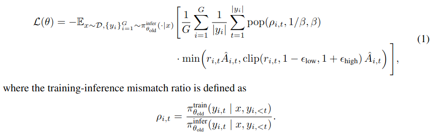
where the pop operator introduces a mask that suppresses samples whos mismatch ratio deviates excessively. This is a Masked Importance Sampling style of algorithmic fix.

Interestingly they use a three policy formulation, using $\pi^{infer}_{old}$ against the old train inference to address mismatch, leaving the PPO clip ratio to only logprobs from the trainer. This goes against much of what I've observed with labs moving to a "bypass" formulation skipping pi_train_old and just using the live infer logprobs to address both train-inference and stale policy mismatch together.

GLM 5.2 Since GLM 5.2 the team has switched from GRPO to a new inhouse developed SAO algorithm: Single-Rollout Asynchronous Optimization.

The motivation was that GRPO forces group wise sampling, which is highly unfit for asynchronous pipelines. Instead they want a algorithm that does away with the group wise sampling. Of course the problem then becomes that you have no baseline function. So instead they bring back the value model, making SAO closer to PPO.

Other

attention topk GLM uses DSA, which uses a indexer to calculate a top-k for sparse attention, producing indexes of which tokens to attend to at each DSA layer. This mechanism runs into similar problems as the expert router does, where discrepancies in training/inference frameworks become exahustrubated if these dont match. top-k matchin is critical for RL stability. For MoE the stock standard approach is communicating the expert indexes between inference and training engines, enabling router replay. However attention indexers have much higher top-k than expert routers, so storing and communicating every index for every token is impractical. GLM finds that adopting a deterministic top-k operator effectively resolves the training-inference mismatch in DSA indexer token selection, compared to non deterministic CUDA based top-k implementation used by SGLang's DSA indexer, directly using native torch.topk is slightly slower but determinstic.

reasoning rl environments math and science is partly curated from data vendors.

They use domain and source specific judge models or evaluation systems to produce binary outcome rewards.

agentic rl environments

Token-in-Token-out is key to eliminate mismatch. This procedure makes sure that as completion tokens are combined with environment tokens that you dont pass through a detoknization stage that may pertrub the ongoing conversation, instead you keep the completions in token space and simply append to it. Prior it was common to detokenize the model output to be able to parse tool calls etc, then retokenize the entire thing, tool call + response and append it to the conversation.

text in text out treats the rollout engine as a black box that returns finalized text; the trainer reconstructs the trajectory by re-tokenizing the text. This seemingly small choice leads to a surprising amount of possible mismatches in token boundaries, whitespace/normalization handling, truncation or special token placement.

GLM team finds TITO to be absolutely crucial for RL training because it preserves exact action-level correspondence between what was sampled and what is optimized.

general rl environments for general rl the team decompose the objective into three dimensions: foundational correctness, emotional intelligence and task specific quality. these are three concrete things they want to optimize for, balanced according to some internal policy. foundational correctness is an important bedrock generally, if the model is not grounded in truth it doesnt matter how well spoken it is, emotional intelligence aims to align the model with the user and communicate as humans do, and task specific quality targets fine-grained optimization across various specific tasks.

given these optimization objectives, how do we then design a reward model to guide learning during general rl? Z.AI use a hybrid reward system to supervise these diverse objectives, containing three complementary reward signals: rule based reward functions, outcome reward models, and generative reward models. rule based provides precise interpretable signals but are limited to aspects expressible as deterministic rules. ORMs offer low variance signals but are suspectible to reward hacking. GRMs leverage language models to produce scalar or structured evaluations, these are less suspeptible to reward hacking, we can define complex grading rubrics etc, but generally these methods are high variance. blending the three gives a nice tradeoff.

a distinct aspect of the general rl pipeline is the incorporation of high quality human authored responses. rather than relying solely on model generated responses they use expert human responses as stylistic and qualitative anchors. this was done after noticing that the model tended to produce very "model-like" patterns in its output - verbose, formulaic, lacking nuance.

on policy cross stage distillation GLM is trained in a sequential multi stage RL pipeline. a natural consequence of this is that sequentially optimizing for distinct objectives can lead to the cumulative degredation of previously acquired capabilities. to mitigate this they finish RL with a on policy distillation stage as the final stage.

slime (synchronous)

to support the widespread set of training stages, different types of RL, ZAI keep working on slime as a unified training stack.

DP attention Conventional attention with multiple KV heads can be nicely parallelised using something like TP. Each rank stores its head of the weights and kv cache. MLA compresses the KV representation into one shared latent vector, making head-wise KV partitioning ineffective. Consequently with TP attention under MLA multiple ranks would process the same sequence typically needing duplicate copies of its latent kv cache. To avoid this GLM does not shard attention at all, instead applying just DP attention. This more effectively makes use of aggregate HBM capacity of 64 GPUs for KV storage.

GLM uses DP64 EP64, so attention, normalization weights are all replicated across ranks, while expert computation is sliced.

tail latency reduction under a synchronous setup it is not aggregate throughput which is the key optimization target for the inference engines but rather end-to-end wall clock latency of the rollout collection phase. Under a sync setup we are forced to wait for the long tails to complete, creating a straggler problem.

GLM employs FP8 rollout inference and MTP to reduce per token latency and shorten the completion time of long trajectories. MTP is especially effective in the long tailed regime of synchronous inference because you naturally always trend towards a small batch decoding regime towards the later part of a rollout collection phase. "Since tail latency is often driven by small-BS stragglers (e.g., rare long contexts, complex multi-turn reasoning, tool-heavy traces), MTP provides disproportionately large benefits on the long tail, improving the time-to-completion of the slowest sample and thus reducing step-level stall time."

slime (async)

to be able to move into agentic engineering, they develop a async variant of the framework, fully decoupling inference from training. inference engines continously generates trajectories. Once the number of generated trajectories reaches a predefined threshold the batch is sent to the training engine to update the model.

GLM 5.2

Compaction RL

GLM 5.2 employs compaction as part of RL training, enabling the model to jointly optimize task execution actions and summarization actions under the same final task reward.

For the inference side of the framework, compaction is very simply, instead of terminating the rollout as we reach the token limit you instead compact the history using the rollout policy, so the current policy creates a summary of the history and then continues working from there. The interesting part is what happens on the training side, because the rollout is no longer a single autoregressive sequence. Let's look closer at how CompationRL compaction works, and then we can look at how training segments are constructed.

After compaction, the context/input prompt is rebuilt as s ⊕ u_resume(S) ⊕ last 2 steps where s is the system prompt, u_resume(S) is a fixed compaction template containing the policy generated summary and the final term keeps the most recent 2 turns while the summary contains only the history preceding the 2 turns. The idea is to preserve long-range information through a lossy summary S_t while retaining recent information exactly. A compaction marks a segment boundary, each segment becomes its own sequence: its own context plus the tokens the policy generated in it (until the next compaction).

So, how do we compute losses over these multi segment sequences? Generally we treat each segment as its own sample, assigning the final sequence reward to all segments in the sequence. The standard logprobs and clipping ratios remain similar, being calculated at a token level. You just have to make sure that if you are going to compute the current trainer side logprobs that you treat each segment as an independant sample.

Cross Segment GAE What about advantage computation? Well the CompactionRL paper uses a PPO style objective, with a GAE formulation as opposed to a group wise sampling scheme. Typically under GAE you want to compute TD residuals. This is done per segment under CompactionRL, where final sequence level outcome reward is assigned to each ending token in the sequence segments. However naively this overcredits actions from early segments, because it looks like the final action of each segment has maximal reward. To solve for this they downweight the final token segment reward strength by how many tokens come after it in the original rollout.

Note that the standard way to compute GAE is to recurse backwards from the last token to the first, calculating the advantage at each position

A_t = δ_t + λ·A_{t+1}

Each token's advantage needs the next token's advantage. This is done recursively for a sequence and in parallel across all sequences in a batch. With compaction a true rollout σ₁ → σ₂ → σ₃, but each segment is a separate sample, σ₁ requires advantages from σ₂, meaning samples cant be computed in parallel. GLM wants to avoid this, so they pretend each segment ends in the real outcome R and sweep every segment independently and in parallel, the fix they do is by introducing one number per segment: λ^{N_{>s}}, where N_{>s} is the number of later tokens. That number depends only on token counts, so it is known. To be clear there is nothing inherent about compaction that requires you to dismiss GAE, GAE can still be fully recoverable, its just an efficiency change to avoid having to recurse across really long rollouts.

GRPO Advantage alternative An alternative to GLMs PPO variant is to just apply standard GRPO under compaction based rollouts. This transition is very seamless, there are very few things that need changing because advantage is broadcast equally to all tokens in the sequence under GRPO, so all you have to do is calculate advantage per sequence based on group statistics and then apply this advantage to all tokens in the segments of each sequence.

Distillation

They describe parallel OPD using more than ten expert models merged into one final checkpoint. It sounds like this is a switch to multi teacher on policy distillation rather than the sequential stages described in the GLM 5 paper.

GLM 5.3

slime supports additional mechanisms like top-p masking to better reproduce the rollout sampling distribution during training, top-k and full vocab OPD. Generally a lot of improvements to slime targeting trainer-inference mismatch. "we added capabilities aimed at RL research: top-p mask, top-k and full-vocabulary OPD, and configurations that improve training–rollout consistency, including R3-style setups and full numerical alignment between the training and rollout paths, which give us finer control over sampling, training, and teacher signals, and make it fast to run controlled comparisons". they report average difference in logprob at the 1e-7 level.

DeepSeek V4

Adopt a specialist training pipeline, training distinct domain specific models with sequential initial fine tuning followed by RL. The specialist are then merged using On Policy Distillation (OPD). Interestingly they train separate experts for different reasoning efforts.

They don't provide much detail, but apparently the V4 series uses Generative Reward Models to evaluate policy trajectories on traditionally hard-to-verify tasks that were previously reliant on human annotation. Per the limited description provided we understand that the policy model acts both as generator and evaluator/judge on its own output, where both models are jointly optimized. " Crucially, we apply RL optimization directly to the GRM itself. In this paradigm, the actor network natively functions as the GRM, enabling the joint optimization of the model’s evaluative (judging) proficiency alongside its standard generative capabilities." Not something I think I've seen elsewhere.

fp4 QAT training FP4 (MXFP4) is applied to two components in the trainer, the MoE expert weights and QK path in the indexer of CSA. Note that they still retain FP32 master weights everywhere from what i can tell. For the expert weights "following the common practice of QAT" the fp32 master weights are quantized to FP4, then dequantized to FP8 for computation. So FP4 QAT to prepare for deployment quantization, and then dequantize to FP8 for efficient matmuls.

As a reminder: FP4 (E2M1): Each $1 \times 32$ block has its own scale factor $s_j$. A weight is represented as $\hat{w} = s_j q$, where $q$ is an FP4 number. FP8 (E4M3): Each $128 \times 128$ block shares a single scale factor $S$.

• Unlike BF16, where each stored value directly represents a weight, scaled FP4/FP8 stores quantized values $q$ alongside shared scaling metadata
• Scale factors are derived during quantization from the original high-precision weights, commonly using absmax scaling: $s = \max(|w|)/q_{\max}$.
• Quantization then maps each weight to $q = \operatorname{round}(w/s)$, reconstructing $\hat{w}=sq$.
• Finer-grained scaling reduces quantization error: With per-tensor scaling, an outlier can stretch the representable range for the entire tensor, reducing precision for other weights. Per-block scaling localizes this effect.
• The tradeoff is increased scale metadata and potentially higher computational overhead.

DeepSeek V4: FP4 uses power-of-two scales, allowing lossless conversion to FP8 when the variation between FP4 sub-block scales fits within FP8's larger dynamic range. This avoids additional quantization error when using FP8 training kernels.

FP4 Inference During inference and rollout they directly use native FP4 quantized weights instead of simulated quantization.

This is very interesting, I'd love to hear more about this with regards to trainer/inference mismatch, cause that means they are running FP4 weights during inference but FP8 computations in the trainer setup, and they are able to do so without trainer-inference mismatch being a problem.

Preemptible and Fault Tolerant Rollout Service There is a task scheduler that can preempt tasks at any point, this combined with hardware failures leads to a desire of having a generation process that is robust to both preemption and fault tolerance. They do this by storing each generated token for a request immediately somewhere in off device memory. During preemption the inference engine is paused and the KV cached saved, meaning a resumed generation can use the stored tokens and kv cache to continue decoding. Even in the event of a fatal hardware error, by continously storing the requests generated tokens they can just re-run the prefill phase to reconstruct kv cache and continue.

Kimi K3

Broadly the RL is scaled across three distinct domains, each encompassing a wide spectrum of sub-tasks, with a single expert for each domain at every reasoning effort level (low, high, max) totalling 9 expert models:

general tasks - general experience, vision, reasoning, faithfulness, search capabilities and knowledge work tasks general agents - long horizon assistant tasks, deep research, paragraph-level writing coding agents - SWE, coding experience, kernel tasks and web dev.

interestingly Kimi actually uses a synchronous RL framework, but slightly modified to get over a couple of the big problems of synchronous schemes. For a given rollout step they will start N rollout tasks, but once M < N tasks have completed they will initiate a training step, so the long tailed rollouts dont hold up resources that are just idle. They then execute the training step synchronously, and once the policy has been updated they proceed with the next step but in the next rollout step you continue rolling out all the rollouts that were underway from the last step, so you still get rollouts under multiple policies, but reduce the cost of stragglers.

reasoning effort RL each problem is associated with an initial token budget $b_o(x)$ estimated from the cold start model. The task reward is overriden with -1 for trajectories whose total token budget exceedes a scaled threshold $\tau b_0(x)$.

agentic generative reward models GRMs are used for non verifiable general tasks. they want an outcome based reward but dont have a rule/verifiable way to calculate such a reward. The GRMs provide outcome level supervision through a generative process. A conventional reward model might encode a prompt-response pair and output a scalar through a regression head. A GRM instead generates an evaluation using language model reasoning.

In K3, the judge follows a mandatory four step procedure, for a group G of rollouts the judge model:

1. Inspect: Read the actual outcome, artifact, or text produced by the agent
2. Generate rubric: formulate evaluation criteria appropriate to the task
3. Score: eval candidate against rubric
4. Scorepad: record criterion-level scores

So the judge model produces a rubric for the task (and hence the rollout group), judges each candidate based on the rubric, then calculates reward through pairwise comparisons of candidates, so unlike in RLVR here the reward for a rollout depends on the quality of other rollouts. This tournament style comparisons provides rewards for each rollout, then you'd calculate advantage as normal.

multi teacher on policy distillation as seen before, K3 adopts a MOPD algorithm to unify the 9 expert models.

MXFP4 QAT MoE expert weight are quantized to MXFP4, with activations computed in MXFP8. Non expert components remain in higher precision. They perform QAT throughout the post-training stage. During RL, rollout and training share the same quantization scheme - eliminating train-inference mismatch.

RL Infra

KV cache offloading. They have a bunch of text just to describe kv cache offloading: "Active decoding blocks remain in GPU KV cache, while reusable idle prefixes are written back to an external KV cache pool in CPU DRAM only when it is evicted from GPU, and is prefetched back before the next reuse."

Adaptive concurrency. As I've talked about extensively in relation to Prime-RL's adaptive concurrency, Kimi K3 actually present this exact behavior and their fix for it. They say that fixed concurrency is difficult to estimate, setting to high leads to KV cache pressure and can trigger preemption. They design an auto-throttling mechanism at the scheduling layer using runtime signals such as active request count, queued requestion count and KV cache utilization to dynamically control how many request are sent to the inference engine. This is exactly what we've explored with adaptive concurrency.

DeepSeek V4.1 Flash

DSV4.1 Flash comes about 5-6 months after the release of V4. Skipping to the post-training section of the paper we read:

In this release, we refrain from introducing novel post-training algorithms. The overall recipe follows the standard paradigm of SFT, RL, OPD, without algorithmic modifications beyond well-established practices. Instead, our efforts are concentrated almost entirely on what the model is trained on rather than how it is optimized

DS has from my perspective been a lab that has heavily focused on the how, and has probably been worse than its chinese competitors when it comes to the what; i've generelly felt that DS has been lacking in the data department, so its very interesting to see them shift focus for this release and seemingly put all focus on data. Again from the paper:

we invest in large scale, automated pipelines for data synthesis and environment construction

We'll get into the details, but essentially just focusing on pipelines to create a diverse set of agentic environments together with reference solutions/reward signals, through solid deduplication, difficulty filtering etc. Lastly to quote the intro of the post-training section again, we'll end off with:

We find that, under a fixed and unremarkable optimization procedure, systematic improvements in the scale, diversity, and verifiability of synthesized data and environments account for essentially all of the observed gains. This observation echoes a broader lesson: at the current stage, the marginal return of engineering the data and environment pipeline substantially exceeds that of algorithmic novelty in post-training.

Which sort of echoes what we've been seeing with RL over the past year, finding ways to scale RL environment leads to remarkable gains in performance across a very broad set of domains, putting in effort in building scalable solutions for this is very high ROI.

Controllable reasoning effort

They introduce a scalar effort level $b$ as an explicit conditioning signal during RL. This is applied to both single turn and multi turn agentic tasks. Specifically they modify the system prompt of a given task with

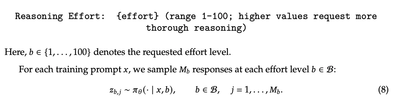
So that means responses sharing the same (x,b) meaning prompt/task and reasoning effort are apart of the same subgroup, used to calculate group based advantage. Responses with different reasoning efforts $b$ are hence not directly comparable. But how does this reasoning effort actually impact learning? Well they do this by introducing a length penalty term in the reward that depends on $b$. At deployment time the scalar $b$ then provides a flexible control interface over the models behaviour, allowing one to shift across the cost-quality frontier. During training only a finite set of effort levels are used, but intermediate values work just as well during deployment as the model has learnt to interpret the scalar. The live API (september) exposes three reasoning efforts low, high, max which map to scalar values 50, 75, 100 respectively.

Asynchronous Post Training Framework

Long-tail is big bottleneck. DS switches completely to an async post-training infrastructure allowing async generation of samples. Per the paper async training is enabled for nearly all of their RL and OPD asks, and rollout efficiency has improved substantially. Again this is the direction I've seen every lab move in, but still Kimi sticks with their synchronous setup.

Bias and Off-policyness Async frameworks come with a few side effects that can degrade training. Firstly it creates a length distribution bias especially in the early training stage because shorter sequences complete first and dominate initial training batches. Second, it creates off policy samples.

DS handles bias via (1) dispatcher limits concurrency on a per-dataset basis which helps regulate the proportion of each dataset in the steady state training batch, which indirectly mitigates length skew by controlling incoming sources, and (2) support for discarding early returned short samples to smooth the transition into steady state length distribution.

For off-policyness (1) control rollout sample dispatch on wait condition for training samples to bound maximum offpolicyness in the rollout engine (2) in training add loss masking scheme that eliminates potentially hurtful token updates with excessive staleness.

Performance optimization stopping rollouts can happen at any token boundary, meaning all in flight samples can stop almost immediately, allowing the system to enter the training phase without delay.

rollout states such as kv, expert routing are persisted at token granularity during generation. upon resumption with a new checkpoint the persisted states are directly reused, eliminating the cost of re-prefilling and allowing interrupted samples to continue exactly where they left off. This is colloqiouly termed "in flight updates".

Xiaomi MiMo V2.6

Algorithm

The algorithm is GRPO-like, using a group wise sampling scheme to calculate advantages, but it doesnt use the PPO clipping, rather looks more like a CISPO style objective

with a importance sampling ratio r calculated between the inference policy and trainer policy. The importance sampling ratio is clipped at four bounds (depending on advantage) giving the mask M. So excessive off policyness token updates are completely masked. So the objective is essentially a token level importance weighted REINFORCE objective with hard masking for excessively off policy tokens.

Grading

For code agent tasks binary rewards from things like test cases provide a scalable correctnes signal, however these signals are indisrinimative for complex tasks, they provide no indication as to implementation quality or problem solving behaviour. To adress this MiMo uses two complementary methods on distinct subsets of the coding tasks.

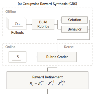
Groupwise Reward Synthesis (GRS) For tasks with high initial pass rate they use multiple offline rollouts to construct task-specific rubrics. An agent studies the task, a bunch of rollouts with the task of turning these into two sets of criteria: solution rubrics, which assess the resulting implementation, and behavior rubrics, which assess how the agent approaches and verifies its work.

Solution rubrics describe what a good implementation looks like, handling of edge cases, consistency with surrounding codebase. Behaviour rubrics describe observable practices that support reliable problem solving, such as gathering relevant evidence and checking the effect of code changes. These rubrics are used to evaluate training rollouts individually, so a agent grader (generative reward model) enters the rollout execution environment and assesses based on task specific rubrics, using resulting code, execution results and trajectory as evidence. It assigns both a solution score and behavior score which is combined with a test score to provide the reward signal.

Groupwise Advantage Resdistribution (GAR) Used for remaining code agent tasks. My understanding is that because these tasks have low passrate they cant construct reliable solution/behavioural rubrics prior to training, so instead they look for a way to enrich the learning signal online. The authors explicitly want a way to discriminate between solutions beyond just correctness, they want to judge quality, maintainability of code etc. So they do this by letting an SFT trained agent (again generative reward model) jointly examine all trajectories in a group, including their patches and test results, ranking them based on

1. Solution approach: Is the chosen approach appropriate for the problem?
2. Precision: Is it implemented correctly, without omissions or unnecessary fallbacks?
3. Minimality: Are the changes limited to what's necessary?
4. Unintended effects: Does the implementation avoid introducing unrelated changes or side effects?
5. Craftsmanship: Does the code follow existing conventions and maintainability standards?

Notice that unlike GRS, which judges trajectories independantly and adjusts the reward, GAR executes a groupwise judging. The judging output is used to redistribute the advantage. They calculate conventional group-relative advantages, then redistribute the positive advantage toward higher-ranked sucessful trajectories. Importantly they redistribute advantage mass, they dont downweight specific trajectories. That means GAR only changes things in a mixed-outcome group. This is unlike GRS which assigns different rewards per trajectory based on rubric scores.

The result of GAR is equal pass rate but with more desirable solutions, fewer turns, less tokens, more maintainable code.

Separate maintainer-oriented audits found that, under pressure to improve test pass rates, policies trained without online grading increasingly adopted undesirable behaviors such as speculative compatibility branches, broad exports, exception swallowing, relaxed validation, and evaluation-specific configuration changes.

Length Penalty

Length penalty is calculated group wise. To start it is only applied if sufficiently many rollouts succeed in the group succeed, then they establish a reference length based the sucessful rollouts. Calculate relative excessive length for all rollouts in the group, w.r.t this reference length. Finally apply a penalty that increases with relative excess length.

Sample Mixer

Across different data sources there is a huge variance in mean generated tokens/active rollout duration. This is tricky because you want the training batch distribution to somewhat match your data distribution despite these large variations so that every data source is trained effectively. The Sample Mixer is the module in charge of solving this issue, it contains a couple of different mechanism.

adaptive rollout concurrency unlike in prime rl, this module is there to balance per source concurrency in the rollout engine such that we are able to maintain a target $B_i$ number of sample groups per training step. This module does so by calculating the expected generation demand and required concurrency based on expected rollout time per source, and then uses that to define the oversampling ratio for the source. so basically this tells the scheduler how many running tasks per source we should maintain such that our training batch has a desired distribution. it builds on the simple observation that maintaining a required completion rate for a slow source requires more concurrent rollouts. So calculation gives us $C_i$, the per source concurrency allowance

adaptive rollout scheduling Now imagine a rollout finishes, freeing up a slot, and multiple data sources have remaining concurrency budget. Which one should we dispatch next?

To determine this they define a scheduling weight per data source, a combination of baseline generation demand and current training batch deficit. So you want to prioritize sources that are missing accepted groups (complete and accepted groups in training batch)

One might ask, why not just maintain $C_i$ per source? This would give you the desired long-run sample distribution. But the problem is that individual batches may still be poorly balanced due to the stochastic rollout durations and filtering. So what MiMo does is add feedback from the actual batch collection progress, instead of just trusting $C_i$ blindly they actually look at how many groups have been accepted. The problem with just going purely by $C_i$ is that you end up with highly fluctuating concurrencies, even though $C_i$ might have been sensible you can end up in a situation where one source completes its target $B_i$ way before another, and then you shift over all concurrency to a slow source which then overshoots its target. So $C_i$ is the budget per source, but the weight is used smooth out the actual live scheduling. The problem is delayed feedback, $C_i$ doesn't know how many groups have completed per sample, so just blindly scheduling $C_i$ will overshoot the target. So there is a combination, you want to schedule according to your desired target, but also adapt to how many groups have actually been accepted.

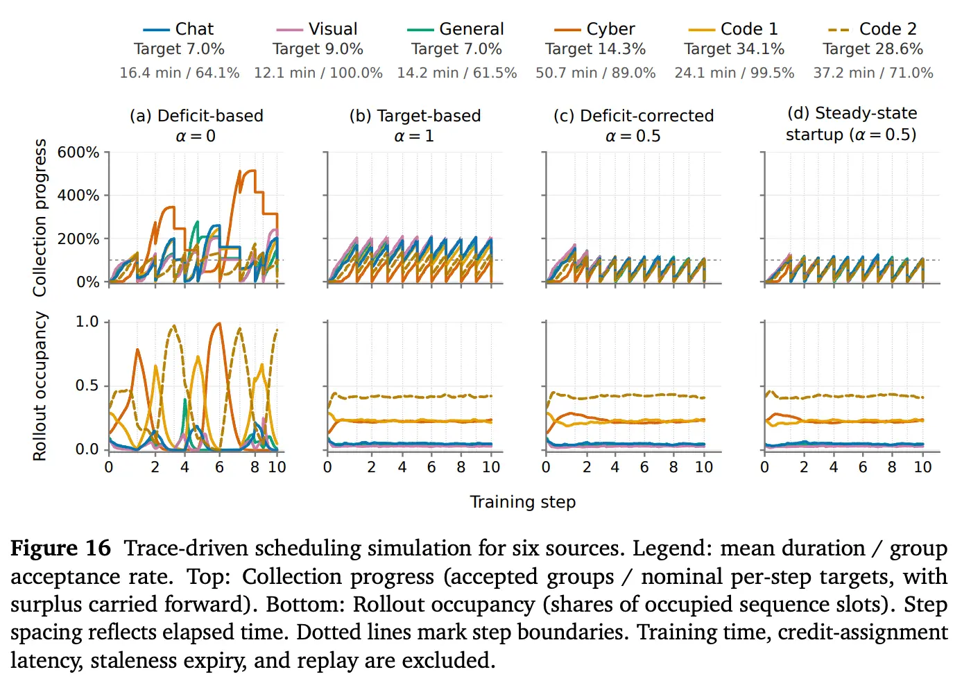
The figure depicts the different mixes deficit-based schedules purely based on how many accepted groups are still needed for the current training batch, while target based schedules purely on fixed proportions determined by the desired training distribution and acceptance rates. Deficit based leads to highly varying rollout concurrency and collection, target based hits a nice steady state rollout distribution, with the proportion of in-flight rollouts belonging to each source settling into a relatively stable distribution. But looking at the accepted groups we see that we still overshoot certain sources quite heavily, because we are not taking into account how many groups have been completed per source. MiMo uses $\alpha = 0.5$ in practice.

predictive rollout dispatch they use per source prior estimates of rollout sequence length to estimate kv demand guiding dispatch across inference engines. this is just a inference router, similar to the likes of vllm-router or llm-d router.

Training/Inference Consistency and Optimization

Apply R3.

Short sidenote on QAT:

---

You maintain full precision weights, but use fake-quantized weights for computation. The output and loss therefor reflect the quantization error. In the backward pass you want to know how to update master weights, so compute loss w.r.t the fake quantized weights

$$\frac{\partial L}{\partial W}=\frac{\partial L}{\partial \hat W}\frac{\partial \hat W}{\partial W}$$

the problem is the second term. Quantization involves rounding, whose derivative is zero almost everywhere and undefined at quantization boundaries, so instead of differntiating through quantization you approximate

$$\frac{\partial \hat W}{\partial W}\approx I$$

In other words, pretend that quantization was the identity function during the backward pass. Consequently

$$\frac{\partial L}{\partial W}\approx\frac{\partial L}{\partial\hat W}$$

---

MiMo says they apply quantize-dequantize (QDQ) to the experts after each parameter update, following the same numeric constraints as MXFP4 Humming used during rollout so the two engines see exactly the same parameters. This is slightly different then QAT, but the details aren't provided to properly understand what MiMo is actually doing. They suggest that they quantize weights to MXFP4 matching rollout engines, but its unclear how these quantized weights interact with the optimizer.

Spec decode They employ block-6 DFlash for spec decode during RL rollout. Initially trained on the SFT policy, DFlash is then finetuned on early RL rollout logs resampled to match the RL training distribution.

RL-adapted FP8 DFlash achieves 10% higher per-node throughput than the baseline.

They dont provide a lot of details on how DFlash acceptence length / verification draft length changes across training.

Building RL Environments

GLM

SWE

Collect large corpus of real-world Issue-Pull Request pairs and apply rigorous rule based and LLM filtering to ensure acquisition of authentic high quality issue statements. The type of issues are bug fixes, refactoring, feature implementation. They include the necessary test requirements to ensure the models' implementation is consistent with the test patch. They use an LLM to extract Fail-to-Pass (F2P) and Pass-to-Pass (P2P) test cases, this essentially means classifying test cases into those that test the bug/feature implementation (F2P) and those which test existing features (P2P) to make sure the gold patch doesnt break anything. Using this methodology they construct 10k verifiable SWE environments

Terminal Environments

There are two ways they form terminal environments, one starts from seed data. Meaning they synthetically generate environments at scale starting from a seed task collected from real-world software engineering and terminal-based computer-use scenarios. It's essentially a synthetic data pipeline that leverages LLMs to brainstorm ideas, create structured task descriptions, Dockerized execution environments and test scripts. The entire environment is generated synthetically, and then passed through a validation loop where it is inspected and refined by other agents according to predefined rubrics.

The other way is synthesis from web-corpus. They search online for high quality web pages containing code relevant information which are ammendable to terminal style task formulation. They then prompt the agent with the Harbor task construction specification alongside each selected web page. The agent synthesizes a complete terminal task grounded in the web page content.

Search Tasks

Construct a web knowledge graph using a search agent that performs semantic parsing for entity recognition, noise filtering and structuted information extraction. Based on the WKG you sample low to mid frequency entities as seed nodes and expand multi hop to form complete subgraphs . A subgraph is then turned into a question answer pair.

Kimi K3

White-box RL environment Training with a single agent harness causes overfitting. Instead they design a unified white box RL environment that represents an abstract agent harness interface as a collection of configurables, composable modules, including tool interfaces, system prompts, context management strategies, skills, memories, subagents etc. Composing these modules through configuration allows the environment to instantiate harnesses such as Kimi Code, Claude Code, Codex, OpenClaw, and Hermes. During RL training they dynamically construct different harness configurations for different task groups.

Knowledge-graph driven task synthesis Generative task synthesis without grounding etc is known to lack diversity and complexity. To better be able to control things like domain coverage, complexity, diversity in task synthesis the team creates a self-evolving hirarchically organized knowledge graph taht agents continously expand through web-scale exploration across knowledge intensive and coding domains.

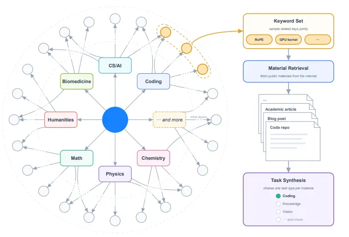
This is demonstrated in the figure. Starting from a couple of diverse seed nodes, agents look through the content of their node and then investigate corresponding concepts in an attempt to expand the graph. This slowly builds a directed acyclic graph through recursive agent-driven expansion. Before adding new nodes agents check that the graph doesnt already contain a similar concept to avoid duplication.

With this knowledge graph available you can sample keyword nodes/concept as a grounding for new task synthesis.

Domains

The paper provides a bit of detail on a bunch of different domains, not as structured as GLMs: SWE, terminal, search. I'll list them here in shortform:

1. Verifiable Agentic Problems - This represents multi-step complex information searching, real day-to-day work of professionals such as investment banking, data analysis and legal practice, multi-step verifiable visual reasoning STEM problems, visual puzzles. The commonality here is that these are agentic environments with well defined verifiability. No details are provided as to how these are sourced
2. Kernel Optimization - Source kernel tasks from high-quality GitHub repos such as Flash Linear Attention. This covers multiple GPU programming languages (CUDA, Triton, CuTe DSL, ThunderKittens and TileLang), widely used GPU architectures and numerical formats. These environments are evaluated through correctness and performance, each kernel provides a PyTorch reference implementation and solutions exceeding a predefined numerical error receive zero reward. Performance is scored against an expert implementation, meaning these tasks are generated from existing kernels (denoted expert implementations).
3. Personal Assistant Tasks - Develop mock implementations of things like Gmail, Notion, Slack, and Canvas that serve as environments for models. Tasks are craeted based on these mock implementations, mimicking real-world professional workflows in scenarios like HR, legal, finance. The agents act in persistent, evolving environment over miltiple simulated days and encounters dozens of interdependent events distributed across applications.
4. Autonomous Execution - These tasks are a bit different, rather than providing a well defined problem/objective, AET generalizes into problems where even the required behaviour may need to be discovered through experimentation. The defining idea of this is verify-in-the-loop optimization. In these tasks, rather than giving the agent a well defined procedure to execute, AET provides: (1) an initial environment state and a goal (2) tools for interacting with and modifying that enviornment (3) a verifier that the agent can repeteadly query for feedback (3) a limited execution and verification budget. The agent must discover how to accomplish the goal, iteratively testing and improving its solution. For example, in the provided example from the paper, the task involves replication of a camera repair management system. Imagine you are given access to an existing application but can not inspect its implementation, and the goal is to build a functionally equivalent system. The agent then needs to query the original application to discover behaviour, implement a replica, submit it to a verifier to test behavior, use diagnostic feedback to identify failures and improve the implementation. Importantly the public verifier provides feedback, while hidden verification on held-out scenarios determines whether the solution generalizes. That helps overfitting to the visible tests.
5. Web Dev - nothing special, quite little info provided

DeepSeek V4.1 Flash

Large Scale Agent Task Synthesis

General Agent uses data from internal employees and external partners where people using the model are encouraged to share interaction and feedback when using the model in their workflows. Based on these interactions DS builds a large set of mocked tools that reproduce the interfaces and behaviours of real-world tools and systems. This covers things like SaaS and enterprise applications as well as more specialized business back end systems. This is used to generate tasks at scale.

Coding agent training environments are built from (1) coding agent sessions from internal employees and external partners, filtered to retain highly complex tasks or tasks where model performance is low, and (2) public GitHub repositories. Environment construction is carried out by multiple collaborating agents. First an agent determines whether the project can be built in a sandbox and verified automatically; if so it selects a specific turn or commit as the task starting point, design several complex implementation details with concrete evaluation points including F2P and P2P test suites. Then another agent is tasked with creating the initial working directory, test code and task descriptions in an isolated container, perform self-testing removing any traces where the solution might leak. So it sets up the environment and runs the first test of it, similar to how a human would test such an environment. Then, multiple distinct agents attempt the task, and an independant quality review agent inspects the environment together with the generated solution traces, checking for environment issues, factual errors, mismatch between eval points and task description, hackability etc.

Through these pipelines DS can batch-produce RL training data that is correct, discriminative, and controllable in length and difficulty.

RL on said synthesized tasks

not too much to say here, very consistent improvement across DeepSWE, TerminalBench, SWEBench Pro as training progresses. They note that they train using a bunch of different agent scaffolds. They also have a small note on the fact that they employ model merging as a way to reinitialize successive RL runs. It seems like they trained a bunch of RL runs separately in parallel while exploring scaffolds, configurations etc, and found that they could quite effectively merge these different runs and keep going.

Xiaomi MiMo V2.6

MiMo details their scaling of RL environments across a number of different domains, I'll go through and outline them separately. The focus is on how to construct environments, task in said environments, and how reward is calculated.

Code Agent Tasks

Task construction comes from a bunch of different sources:

1. GitHub - pull requests and issues, if a pull request is missing or has a bad issue they attempt to reconstruct an issue style spec via LLM
2. Everyday dev workflows - collected from "vibe coding" by internal employes, this can be anything from feature implementation, refactoring, debug etc
3. Spec driven tasks - a bit unsure what this is they describe it as tasks that emphasize code generation under detailed multi-constraint requirements
4. Sourc code driven - use CodeMidas to derive tasks from functionality in existing codebases. agents identify candidate functionality and translate its observable behaviour into task specs and executable environemnts. kind of like the github way but without a need for issues, PRs etc.
5. Data vendors

Supervision Tasks are reviewed for sufficient coverage. An overarching goal is to accept implementations that satisfy the spec and reject those that violate it, withour requiring incidental details of a reference implementation. Each task is attempted 4 times by a coding agent. An audit agent receives the 4 rollouts along with problem statement, tests, reference path, etc. The auditor tries to articulate what a correct solution requires and assesses whether the tests capture those requirements, then it evaluates each submitted solution against the spec in a workspace. The idea is to look at solutions, how they were judged, and try to identify holes in the task, look for mismatch between task intended behaviour and the implemented verification.

Naturally they use F2P and P2P tests.

General Agent Tasks

A general agent environment is a workspace and a set of software tools, accessible through interfaces such as MCP, API, CLI, GUI. They build large local rich environments by replicating system behaviours, collecting real world files, software mocks. These environments are assembled via a planning agent that specifies the workspace/environment structures, selects appropriate tools and plans files and database contens. Web search grounds the plan in real world information, while relationships across files and between files and database records supports subsequent multi hop reasoning and cross validation. Many agents generate files and populate the environment in parallel following the shared plan. Finally a review agent checks the artifacts and global consistency.

After building said environments, ideally rich and vast, you can then generate a bunch of tasks for them. MiMO survey common professional tasks and combine and generalize them into seed tasks. An agent explores each environment, using the seeds to construct tasks suited for the environment and tools. Task completion is evaluated using atomic, binary rubric items: code-based checks verify deterministic properties such as database values and deliverable formats while LLM based checks asses open ended content.

Cybersecurity Agent Tasks

OSS-Fuzz supplies tens of thousands of manually confirmed instances of a project and a target bug. They use these to task an agent to construct the input that triggers it. Importantly the difficulty is not triggering a crash but triggering the specific vulnberability described. Verification must therefore spearate the intended bug from unrelated crashes.

For each vulnerability they check out the source at the reported commit, build the fuzzing harness and give the agent the complete runtime environment.

Reward Hacking Mitigation

During mid-training they introduce data where MiMo reflects on the faulty reasoning, revises the relevant turn and continues with actions grounded in the task spec. Goal is to improve model alignment.

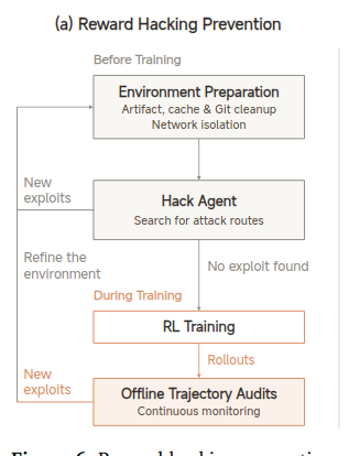
RL environments have a risk of containing the existing solutions. Building a project with the reference patch applied (which is typically done during environment construction to verify patch works and correctly passes tests) can leave behind artifacts. Remove build logs, verifier outputs, residual patches. Also need to be careful about Git history containing the later commits which contain solution.

They also apply a a hack agent that probes the environments for remaining leaks and weaknesses. These agents help find new exploit paths that can be added to environment prep. Iteratively hack agents can help improve the environment prep to reduce risk of hacking.