linear attention and its gated descendants

a brief history on linear attention. from its original to the deltanet variants that are increasingly popular in todays open frontier.

---

Before we get into linear attention at all, lets start by realising some of the issues of standard softmax attention Transformers:

1. During training we have quadratic time complexity in sequence length.
2. During inference (memory bound) we have linear memory complexity as the KV cache memory storage grows linearly with each token leading to high memory burden hence increasing latency.

Standard Softmax Attention

For a sequence of length L with hidden dimension d, causal attention computes:

$$O = \mathrm{softmax}(QK^\top + M)V$$

where:

• $Q, K, V \in \mathbb{R}^{L \times d}$
• $M$ is the causal mask
• $QK^\top \in \mathbb{R}^{L \times L}$

The causal mask means token $t$ can only attend to tokens $\le t$.

Complexity:

$$QK^\top: O(L^2d)$$ $$\mathrm{softmax}(QK^\top)V: O(L^2d)$$

So total time is:

$$O(L^2d)$$

Memory during training is also sequence-quadratic because the attention matrix is $L \times L$.

Without Softmax and Masking

If attention did not have softmax and causal masking, we would like to reassociate:

$$Q(K^\top V)$$

instead of:

$$(QK^\top)V$$

The latter forms an $L \times L$ matrix; the former first forms a $d \times d$ matrix.

But softmax attention is:

$$\mathrm{softmax}(QK^\top + M)V$$

The softmax and causal mask operate on pairwise token-token scores, so we cannot freely move parentheses and turn the whole operation into $Q(K^\top V)$.

Linear Attention as a Linear RNN

A conventional RNN usually has a nonlinear state transition:

$$h_t = \phi(W_hh_{t-1} + W_xx_t + b)$$

A linear, or more exactly affine, RNN has a transition like:

$$h_t = A_th_{t-1} + b_t$$

The word "linear" refers to the dependence on the previous recurrent state. It does not mean the whole model is a linear function of the input tokens.

Linear attention is a linear RNN with a matrix-valued state. Using column vectors for individual tokens:

$$S_t = S_{t-1} + v_tk_t^\top$$ $$o_t = S_tq_t$$

The state is:

$$S_t = \sum_{i \le t} v_ik_i^\top$$

So $S_t$ is an accumulated key-value memory. Each token writes a rank-1 matrix into the state, and the current query reads from that state.

This flips the usual RNN tradeoff:

standard RNN:      O(d)-sized state,   O(d^2) recurrent transform
linear attention: O(d^2)-sized state, O(d^2) rank-1 update/read

The important trick is that linear attention gets a $d \times d$ state without using a dense $d^2 \times d^2$ transition matrix. A dense transition over a $d^2$-sized state would cost $O(d^4)$. The outer-product update costs only:

$$v_tk_t^\top: O(d^2)$$

One nuance: for vanilla linear attention, the additive states are prefix sums in principle:

$$S_t = X_1 + X_2 + \cdots + X_t,\qquad X_i = v_ik_i^\top$$

So the recurrent presentation is not the only possible training implementation. But the token-by-token recurrent form is the natural decoding view, and the chunkwise form is the hardware-practical training/prefill view.

For batched chunk notation below, $Q_{[i]}, K_{[i]}, V_{[i]}$ are row-major matrices in $\mathbb{R}^{C \times d}$. With this convention, applying a state to all queries in a chunk is written as $Q_{[i]}S_{[i]}^\top$.

Recurrent Linear Attention for Inference

During autoregressive generation, softmax attention with a KV cache still has to scan all previous tokens at every step.

At step $t$:

$$q_tK_{\le t}^\top: O(td)$$

and the weighted value sum is also:

$$O(td)$$

So per generated token:

$$O(td)$$

Across L generated tokens:

$$\sum_{t=1}^{L} O(td) = O(d)\sum_{t=1}^{L}t = O(L^2d)$$

The KV cache avoids recomputing old keys and values, but it does not avoid reading over them.

For recurrent linear attention, each new token updates:

$$S_t = S_{t-1} + v_tk_t^\top$$

and computes:

$$o_t = S_tq_t$$

Per token:

$$v_tk_t^\top: O(d^2)$$ $$S_tq_t: O(d^2)$$

So across L generated tokens:

$$O(Ld^2)$$

Memory changes from storing the full KV cache:

$$O(Ld)$$

to storing one state matrix:

$$O(d^2)$$

Key inference win: no sequence-length scan during decoding. Each new token pays fixed cost with respect to context length.

Recurrent Form for Training

The recurrent form is natural for decoding, but awkward for training/prefill.

Naively, training would require:

$$S_1 \rightarrow S_2 \rightarrow \cdots \rightarrow S_L$$

with one update per token:

$$S_t = S_{t-1} + v_tk_t^\top$$

and one output per token:

$$o_t = S_tq_t$$

The theoretical complexity is:

$$O(Ld^2)$$

which can look good asymptotically. But the computation has two practical problems:

• Dependency chain length is L, so parallelism is poor in the naive recurrent implementation.
• The operations are many small rank-1 outer products ($v_tk_t^\top$) and matrix-vector products ($S_tq_t$), which are inefficient on GPUs compared with dense matmuls.

This is the main distinction: theoretical complexity and actual hardware performance are not the same thing.

Chunkwise Parallel Form

Chunkwise parallel form is the training/prefill compromise between two bad extremes.

The full parallel causal form has a good GPU shape, but it is still quadratic in sequence length because causal masking forces explicit token-token interactions:

$$(QK^\top \odot M)V: O(L^2d)$$

The fully recurrent form is theoretically linear in L, but exposes a length-L dependency chain and many small rank-1 / matrix-vector operations:

$$S_t = S_{t-1} + v_tk_t^\top,\qquad o_t=S_tq_t$$

The chunkwise idea: do not process one token at a time, and do not process the whole sequence as one masked attention matrix. Process blocks.

Break the sequence into chunks of size C, giving about:

$$L/C$$

chunks.

The algorithm has two steps:

1. compute the recurrent state at chunk boundaries
2. compute token outputs inside each chunk

Chunkwise does not remove recurrence. State computation is still sequential across chunks; it reduces the chain from L token steps to L/C chunk steps.

Step 1: Chunk-Boundary State

The state is computed only at chunk boundaries:

$$S_{[i+1]} = S_{[i]} + V_{[i]}^\top K_{[i]}$$

where $V_{[i]}, K_{[i]} \in \mathbb{R}^{C \times d}$.

This works because the linear attention state is additive:

$$S_b = S_a + \sum_{t=a+1}^{b} v_tk_t^\top$$

and the chunk sum of rank-1 updates is one matmul:

$$\sum_{t=a+1}^{b} v_tk_t^\top = V_{[i]}^\top K_{[i]}$$

Cost per chunk:

$$V_{[i]}^\top K_{[i]}: O(Cd^2)$$

Across $L/C$ chunks:

$$O((L/C)Cd^2)=O(Ld^2)$$

This is the same total arithmetic order as token-wise updates, but packaged as larger matmuls.

Step 2: Output Compute

For each chunk, split the output into:

$$O_{[i]} = \text{previous-chunk contribution} + \text{within-chunk contribution}$$

Every token in the current chunk can see all previous chunks. That history is summarized by the boundary state $S_{[i]}$:

$$Q_{[i]}S_{[i]}^\top$$

Cost per chunk:

$$O(Cd^2)$$

Across all chunks:

$$O((L/C)Cd^2)=O(Ld^2)$$

Tokens inside the current chunk still need causal masking relative to each other. But the mask is only $C \times C$, not $L \times L$:

$$(Q_{[i]}K_{[i]}^\top \odot M_C)V_{[i]}$$

Cost per chunk:

$$Q_{[i]}K_{[i]}^\top: O(C^2d)$$ $$(QK)V: O(C^2d)$$

Across all chunks:

$$O((L/C)C^2d)=O(LCd)$$

So the chunkwise output is:

$$O_{[i]} = Q_{[i]}S_{[i]}^\top + (Q_{[i]}K_{[i]}^\top \odot M_C)V_{[i]}$$

Total chunkwise cost:

$$O(Ld^2 + LCd)$$

If C is much smaller than L, this is subquadratic in sequence length and much better than:

$$O(L^2d)$$

The limiting cases are useful:

• C = 1: recurrent form, maximally sequential, $O(Ld^2)$
• C = L: full parallel masked form, $O(L^2d)$
• intermediate C: block matmuls plus chunk-level recurrence

That is the appeal of chunking: it converts a long stream of small operations into dense GEMMs plus state transfer between blocks. The algorithm is more intricate than standard attention, so real performance depends on kernel quality and benchmarking, not just big-O.

mental model

Softmax attention:

all tokens x all tokens
good GPU shape, but quadratic in sequence length

Recurrent linear attention:

token -> token -> token -> token
linear in sequence length, great for decoding, poor GPU utilization for naive training

Chunkwise linear attention:

chunk -> chunk -> chunk
inside each chunk: parallel dense matmuls
between chunks: compact recurrent state

In practice chunk size C is typically set to {64, 128, 256}. The chunkwise parallel algorithm can be generalized to linear attention with decay and delta rule. It is the defacto standard for training modern linear attention models including Mamba2, GLA, Lightning Attention, DeltaNet and others.

Hardware Performance

Songlin comments on the speedup achieved after implementing both the recurrent and chunkwise version in Triton:

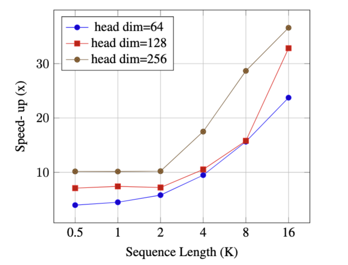
chunkwise parallel approach consistently outperforms the recurrent baseline...this performance advantage grows more pronounced under two key conditions: as sequences get longer and as head dimensions increase.

Why? Songlin points to two issues (1) existing recurrent implementations process token-by-token, relying instead on both batch and head dimension to saturate GPU cores:

While this strategy worked well with moderate sequence lengths and larger batch sizes, it faces challenges in modern training scenarios. Today's models increasingly work with longer sequences or larger model parameters, often necessitating smaller batch sizes for memory efficiency. This shift was notably highlighted in the FlashAttention2 paper, which identified sequence-level parallelism as crucial for training.

when batch size x head dim is small, there isn't enough parallel work to keep modern GPUs fully utilized.

(2):

Tensor cores are designed around matmuls offering up to >16x speedup compared to other operations with equivalent FLOP counts. Recurrent implementations, despite requiring fewer total FLOPs, struggle to effectively leverage these hardware accelerators...Our chunkwise implementation, in contrast, restructures the computation to maximize use of tensor cores, achieving better real-world performance despite higher theoretical FLOP counts. This performance analysis illustrates a crucial principle in modern hardware-efficient deep learning: raw FLOP counts don't always translate directly to wall-clock time. The ability to leverage specialized hardware accelerators and maintain high GPU utilization often matters more than theoretical operation counts.

Linear Attention Takeaway

Linear attention's key move is replacing explicit token-token attention with an accumulated key-value state:

$$S_t = \sum_{i \le t} v_ik_i^\top$$

This gives excellent autoregressive inference behavior because the model no longer scans the full context for every generated token.

For training/prefill, the pure recurrent form is too sequential in its naive form. Chunkwise parallel form combines the recurrent and parallel views:

• recurrent across chunks
• parallel inside chunks
• dense matmuls instead of many tiny outer products
• complexity roughly $O(Ld^2 + LCd)$

The practical lesson is that asymptotic complexity is only part of the story. Chunkwise linear attention is a hardware-aware algorithm: it accepts a bit of extra theoretical work to expose parallelism and tensor-core-friendly matmuls.

Gated variants of Linear Attention

Unfortunately, despite the aforementioned possibilities of performance efficiency improvements, in the end the language modeling capabilities of Linear Attention fall well short of their Transformer counterparts. There's no free lunch. Compressing history into a fixed size state matrix means we cannot perfectly preserve all historical context, by design. More formally, linear attention implements a key-value associative memory, which is the sum of outer products between keys and values $S = \sum v_ik_i^\top$. This space is inherently limited by $d$. We don't have enough "room" to store all our prevous keys. We run into memory overload: in this key-value associative memory system, we can only add new key-value associations without the ability to erase existing information. As sequences grow longer, this leads to accumulating "retrieval errors" that degrade performance.

To address this limitation research moved to finding ways to incorporate forgetting mechanisms.

linear attention with data-independent decay

One of the most obvious things would be to realize that generally, distant tokens are less important than recent ones, so just add a decay factor to the state:

$$S_t = \gamma S_{t-1} + v_tk_t^\top$$

where $0 < \gamma < 1$. This works quite well in practice, was used by MiniMax in their Lightning Attention. This is a simple exponential moving average of the state.

linear attention with data-dependent decay

the previous variant uses a fixed decay rate, independent of the input data. however we can imagine that for different positions we want the model to have flexibility of adjusting the decay rate and that how you end up with data-dependent decay rates.

$$S_t = \gamma_t S_{t-1} + v_tk_t^\top$$

Here we say that $\gamma_t$ is data dependent, meaning that it is a function of the input data $x_t$. For example you could have a linear projection of $x_t$ to compute gamma, in the same way q,k,v are computed.

This type of decay is employed in Mamba2, mLSTM and more.

linear attention with fine-grained decay

We can imagine a more fine-grained decay mechanism. While $\gamma$ was a simple decay scalar work like GLA uses a more fine-grained d x d matrix to decay the state

$$S_t = G \odot S_{t-1} + v_tk_t^\top$$

To summarize this section:

• Language modeling has strong recency bias
• Decay helps bridge perplexity gap between linear attention and softmax attention
• Fine-grained decay improves performance but faces scaling issues. Outer-product based decay structures are required to enable chunkwise forms as set up earlier

DeltaNet

Towards an even more expressive update rule.

The previous decay variants add forgetting, but they still do not directly solve the key-value memory problem. Vanilla linear attention is append-only:

$$S_t = S_{t-1} + v_tk_t^\top$$

Every new key-value association is added to memory, whether or not a similar key already exists. This muddies the memory as we accumulate overlapping associations.

The associative memory view makes this clear. Since:

$$S = \sum_i v_ik_i^\top$$

retrieving with a key/query-like vector $k$ gives:

$$Sk = \sum_i v_i(k_i^\top k)$$

For example, with multiple entries:

$$S = v_1k_1^\top + v_2k_2^\top + \cdots$$

Querying with $k_2$ gives:

$$Sk_2 = v_1(k_1^\top k_2) + v_2(k_2^\top k_2) + \cdots$$

If keys are normalized and roughly orthogonal:

$$k_2^\top k_2 \approx 1,\qquad k_i^\top k_2 \approx 0 \text{ for } i \ne 2$$

so:

$$Sk_2 \approx v_2$$

If keys were perfectly orthogonal, then querying with $k_j$ would isolate $v_j$. In reality keys live in limited $d$-dimensional space, so they interfere. The state matrix has finite capacity and memory quality degrades as more associations are added. The model has no way of solving this by itself, it is forced into "memory overload".

DeltaNet changes the update from unconditional addition to an error-correction rule:

$$S_t = S_{t-1} + \beta_t(v_t - S_{t-1}k_t)k_t^\top$$

Here $S_{t-1}k_t$ is what the current memory already retrieves for key $k_t$. This is the "prediction" in the delta rule sense. $v_t$ is the target value we want memory to return for this key.

So DeltaNet says: look up the old value for this key, compare it with the new value, and write the correction rather than blindly adding the full value again.

Let:

$$v_{\text{old}} = S_{t-1}k_t$$

Then:

$$S_t = S_{t-1} + \beta_t(v_t - v_{\text{old}})k_t^\top$$

This can be interpreted as erase + write:

$$v_{\text{new}} = (1-\beta_t)v_{\text{old}} + \beta_t v_t$$

and:

$$S_t = S_{t-1} - v_{\text{old}}k_t^\top + v_{\text{new}}k_t^\top$$

So $\beta_t$ controls how strongly the new value overrides the old retrieved value:

• $\beta_t = 0$: keep old memory
• $\beta_t = 1$: fully replace the retrieved value with $v_t$
• $0 < \beta_t < 1$: blend old and new

The important conceptual move:

vanilla linear attention: append-only associative memory
DeltaNet: editable associative memory

This connects directly to the no-free-lunch problem. Since the state matrix has limited capacity, we need a better policy for using that capacity. DeltaNet makes the write operation depend on what is already stored, using the prediction error to update memory more carefully.

Gated DeltaNet

Gated DeltaNet is a simple extension of DeltaNet that adds a Mamba2-like decay gate to the state update.

Recall Mamba2-style gated linear attention:

$$S_t = \alpha_t S_{t-1} + v_tk_t^\top$$

where $\alpha_t \in (0,1)$ is a data-dependent gate that controls how much old state is preserved.

DeltaNet instead performs targeted memory editing:

$$S_t = S_{t-1}(I - \beta_t k_tk_t^\top) + \beta_t v_tk_t^\top$$

Gated DeltaNet combines these:

$$S_t = S_{t-1}\left(\alpha_t(I - \beta_t k_tk_t^\top)\right) + \beta_t v_tk_t^\top$$

Equivalently:

$$S_t = \alpha_t S_{t-1} + \beta_t(v_t - \alpha_t S_{t-1}k_t)k_t^\top$$

So the prediction is now made from the decayed previous memory:

$$\alpha_t S_{t-1}k_t$$

Kimi Delta Attention

Kimi Delta Attention (KDA), used in Kimi Linear and Kimi K3, is best understood as a refinement of Gated DeltaNet.

The main conceptual change is:

Gated DeltaNet: one forget gate per head
KDA: one forget gate per key channel inside each head

Before writing the KDA update, it is useful to make the multi-head structure explicit. Linear attention variants still fit into the usual multi-head attention architecture:

x_t
 -> project to q, k, v for each head
 -> each head runs its own recurrent state update
 -> concatenate head outputs
 -> output projection

For one head:

$$q_t,k_t \in \mathbb{R}^{d_k},\qquad v_t \in \mathbb{R}^{d_v}$$

and the recurrent state is:

$$S_t \in \mathbb{R}^{d_k \times d_v}$$

This follows the Kimi paper convention, where the output is read as:

$$o_t = S_t^\top q_t$$

So each head has its own associative memory. If there are $H$ heads, the total state per layer is:

$$H \times d_k \times d_v$$

not:

$$d_{\text{model}} \times d_{\text{model}}$$

This is important because it keeps the recurrent state manageable.

In Gated DeltaNet, the forget gate is a scalar per head:

$$\alpha_t \in (0,1)$$

and the update is:

$$S_t = \alpha_t(I - \beta_t k_tk_t^\top)S_{t-1} + \beta_t k_tv_t^\top$$

This means the whole memory matrix for that head is decayed by the same amount.

KDA changes $\alpha_t$ from a scalar into a vector:

$$\alpha_t \in (0,1)^{d_k}$$

and applies it as a diagonal matrix over the key/address dimension:

$$\mathrm{Diag}(\alpha_t) \in \mathbb{R}^{d_k \times d_k}$$

making KDA's recurrent form:

$$S_t = (I - \beta_t k_tk_t^\top)\mathrm{Diag}(\alpha_t)S_{t-1} + \beta_t k_tv_t^\top$$

The clean way to read this is in two stages.

Decay Old Memory

$$\bar{S}_{t-1} = \mathrm{Diag}(\alpha_t)S_{t-1}$$

This scales the rows of $S_{t-1}$, meaning each key/address channel gets its own forgetting rate:

key channel 1: decay by alpha_1
key channel 2: decay by alpha_2
key channel 3: decay by alpha_3
...

Apply Delta-Rule Update

Then apply the usual delta-rule correction to the decayed memory:

$$S_t = \bar{S}_{t-1} + \beta_t k_t(v_t - \bar{S}_{t-1}^\top k_t)^\top$$

So the prediction is not made from the raw old memory. It is made from the already-forgotten memory:

$$v_{\text{old}} = \bar{S}_{t-1}^\top k_t$$

Then KDA writes the error correction:

$$\beta_t k_t(v_t - v_{\text{old}})^\top$$

This gives $\alpha_t$ and $\beta_t$ separate roles:

• $\alpha_t$: what old memory survives into this step
• $\beta_t$: how strongly the new association is written

where does this leave us?

A good layered understanding is:

1. Linear Attention Memory is append-only:

$$S_t = S_{t-1} + k_tv_t^\top$$

2. DeltaNet Memory becomes editable via prediction-error correction:

$$S_t = (I-\beta_tk_tk_t^\top)S_{t-1} + \beta_tk_tv_t^\top$$

3. Gated DeltaNet Memory gets a forget gate:

$$S_t = \alpha_t(I-\beta_tk_tk_t^\top)S_{t-1} + \beta_tk_tv_t^\top$$

4. KDA Forgetting becomes channel-wise:

$$S_t = (I-\beta_tk_tk_t^\top)\mathrm{Diag}(\alpha_t)S_{t-1} + \beta_tk_tv_t^\top$$

The important structural shift is that from DeltaNet onward, the state update is no longer only additive. Vanilla linear attention has:

$$S_t = S_{t-1} + B_t$$

DeltaNet, Gated DeltaNet, and KDA have multiplicative state transitions:

$$S_t = A_tS_{t-1} + B_t$$

where for KDA:

$$A_t = (I-\beta_tk_tk_t^\top)\mathrm{Diag}(\alpha_t)$$

Now each token does not merely add something to the state. It also transforms the previous state before writing. Important to remember that the chunkwise parallel form remains integral to be able to implement these attention variants.