breaking down dspark and its lineage

Autoregressive decoding is memory-bound. Generating one token requires streaming every weight in the model through the accelerator, and the arithmetic performed against those weights is trivial by comparison. The hardware sits mostly idle waiting on memory. Yet the same forward pass, handed a block of tokens instead of one, costs almost the same wall-clock time. Speculative decoding is the exploitation of exactly that asymmetry: guess several tokens cheaply, then spend one target-model forward pass checking all of them at once.

Recently published DSpark is DeepSeek's take on this and is deployed in their V4 serving system. Reading it, what stands out is how much of it is inherited. Almost every component has a clear ancestor in work from the last two years, and the paper is easier to appreciate once you have seen where those pieces came from. So this post walks the lineage first, from Medusa through EAGLE and MTP to diffusion drafting, and arrives at DSpark at the end.

I hadn't really been following speculative decoding. It's one of those lines of work I'd largely ignored for the past few years, filed under "someone else's problem." Then DSpark came out a few weeks ago and it seemed like an appropriate time to actually understand what's going on here. Reading the paper, I quickly realised that I was out of my depth, and that I had to backtrack to really understand what was going on. Nearly every piece in DSpark has a clear ancestor somewhere in the last two years of work, and the paper is a lot easier to appreciate once you've seen where those pieces came from. So, naturally I went back to try and trace the linearge, and this post is roughly what I ended up with.

Speculative decoding basics: drafting and verification

Speculative decoding builds on a simple idea: guess a possible continuation to the sequence, then verify if the continuation was correct in the next forward pass. If the target model thinks the draft tokens are likely enough (we'll get back to what enough means), we accept them and continue generating from there. The guessed tokens are typically referred to as draft tokens, and the better the drafter (the model used to guess) the greater the speedup.

To be a bit more formal about things: assume a target distribution $p$ (the model we want to sample from) and a draft distribution $q$ (something cheap). The drafter proposes $\gamma$ tokens autoregressively:

$x_1, x_2, \dots, x_\gamma$

costing $\gamma$ sequential cheap passes. The target then takes the whole concatenation at once:

$[\text{prefix},\ x_1,\ x_2,\ \dots,\ x_\gamma]$

Under a causal mask, position $k$'s output depends only on tokens $\le k$. So a single forward pass emits, in parallel, every conditional we need:

$p(\cdot\mid \text{prefix}),\quad p(\cdot\mid \text{prefix}, x_1),\quad \dots,\quad p(\cdot\mid \text{prefix}, x_1{:}x_\gamma)$

That is $\gamma+1$ distributions for the price of one forward pass instead of $\gamma$. The drafter is, in effect, a sampler, and the target is a verifier.

Preserving the target distribution during verification

That single forward pass leaves us with the target's distribution at every draft position, and we need a rule for turning those into accept/reject decisions.

The tempting rule is a threshold: keep the draft token whenever the target also assigns it reasonable probability. It is fast and it mostly works, but what comes out is neither $p$ nor $q$, it is a threshold-dependent blend of the two, and the blend shifts with the sampling temperature and with how well the drafter happens to track the target on a given prompt. You would be shipping a different model than the one you evaluated, in a way that is hard to characterize and harder to debug.

The rule we actually want is one that emits tokens distributed exactly as $p$, despite having drawn $x$ from $q$, so that turning speculation on is invisible in the outputs.

It helps to picture $p$ and $q$ as bar charts stacked over the vocabulary:

token:        0       1       2
p (target):  0.5     0.3     0.2
q (draft):   0.4     0.5     0.1

overlap=min: 0.4     0.3      0.1     ← sum 0.8   the part they AGREE on
p sticks up:  0.1     —       0.1     ← sum 0.2   target wanted MORE here
q sticks up:  —       0.2     —       ← sum 0.2   draft over-eager here

The overlap is the mass the two distributions share. Where the draft proposed a token no more often than the target would have, the draft's sample is already a valid sample from that shared region and we can simply keep it. Where the draft proposed a token more often than the target would have, keeping every such sample would over-represent it, so some fraction has to be discarded. That gives two cases:

1. $p(x) \ge q(x)$: always accept. The target endorses the token at least as strongly as the draft proposed it, so keeping it is honest.
2. $p(x) < q(x)$: the draft was over-eager. Accept with probability $p(x)/q(x)$, otherwise reject and resample from the normalized residual, the "$p$ sticks up" mass in the diagram.

The residual is exactly the mass the draft under-proposed, so resampling from it fills in precisely what the accept step left out. Case 1 contributes the shared mass, case 2 keeps the right fraction of the over-proposed tokens, and the rejection branch supplies the deficit, which sums over the vocabulary to $p$. In short, keep the draft's guess unless the target liked it less than the draft did, and in that case keep it in proportion to how much less.

Speculative decoding is therefore lossless in distribution, a pure systems optimization, and every method in this post inherits that property. Which is also why the drafter can be as crude as you like without any correctness consequence, a point that becomes load-bearing later on.

Latency

With the output distribution pinned, speed is the only thing left to optimize, and it is governed by one equation, written here as in the DSpark and DFlash paper:

$L = \frac{T_{\text{draft}} + T_{\text{verify}}}{\tau}$

Latency per emitted token is drafting time plus verification time, divided by $\tau$, the mean number of tokens accepted per cycle. A drafter has exactly two levers: make $T_{\text{draft}}$ smaller, or make $\tau$ larger. The two trade against each other, since spending more compute on drafting generally buys better guesses and higher acceptance, and every method below is a different bet about where to sit on that trade. Spend more compute drafting and you generally get better guesses and a higher $\tau$; spend less and $T_{\text{draft}}$ falls but so does acceptance.

Medusa - deleting the draft model

The original formulation takes the setup above literally: the drafter is a second, smaller language model from the same family, run alongside the target. A 7B target might be paired with a 68M draft model, which proposes a few tokens, and the 7B verifies them. It works, and as established above the distribution guarantee holds regardless of what the small model does, which is a large part of the appeal.

The difficulties are practical rather than theoretical. Finding a good draft model is hard, since you need something small enough to be cheap and aligned enough with the target to be accepted, and those pull in opposite directions. Not every model family ships a small sibling, and when one exists it was trained for its own sake rather than to mimic a larger relative. Then, having found one, you have to serve two separate models side by side, with their own weights, their own KV caches, and their own memory budget. The conceptual simplicity of speculative decoding is undone by operational complexity.

Medusa is one of the early works that removes the separate model altogether by folding the drafter into the target. Rather than running an independent network, the drafter becomes a small extension of the model you were already serving, so there is one set of weights, one KV cache, and one forward pass.

The mechanism rests on an observation about what the target model already computes. During a normal forward pass, the last hidden state at position $t$, the vector immediately before the LM head, is the model's fully contextualized summary of everything it has read so far, and the model uses it to predict token $t{+}1$. But that vector is not narrowly about the next token. It is a rich, deep representation of the context, and it carries information about how the sequence is likely to continue well beyond one step, which the target's LM head simply never asks for.

Medusa asks for it by bolting $K$ additional small heads onto that same final hidden state, each a lightweight feedforward layer plus a projection to vocabulary size. In the same forward pass that produces the normal next token, those heads read the same vector and each predicts a different future position:

• the target's own LM head: position $t{+}1$ (the real output)
• Medusa head 1: position $t{+}2$
• Medusa head 2: position $t{+}3$
• head $K$: position $t{+}K{+}1$

The heads are trained on the frozen target with the base model's own outputs as supervision, which is cheap compared to training a draft model from scratch. At inference, one forward pass yields the real next token plus $K$ guesses at the tokens after it, with no second model to serve and no extra weight streaming beyond the heads themselves.

Note what the shared input implies. Every head reads the same hidden state, the one computed for position $t$, and all $K$ of them run in parallel within that single pass. Head 2 predicts token $t{+}3$ having never seen what token $t{+}2$ turned out to be, because $t{+}2$ was being guessed simultaneously by head 1. Each head produces its own marginal distribution over its own position, and nothing ties them together into a coherent sequence: the heads predict without inter-token dependency, giving independent marginals rather than a joint. This shows up as acceptance that decays quickly down the block, and it is the property most of the later work is reacting to.

Tree attention

Independent marginals cut the other way too. If head 2 does not know what head 1 chose, then head 1's single top choice is a fragile thing to build on, and committing to one continuation per position means a single early mistake wastes the whole block.

Medusa's authors measured this directly: top-5 accuracy on their heads reached roughly 80% where top-1 was around 60%. The right token is usually in a head's shortlist even when it is not the head's first choice, which argues for proposing several candidate continuations rather than one and letting the target decide which survives.

So each head emits its top-$k$ tokens instead of just its argmax, and candidate sequences are formed as a Cartesian product across heads, pairing head 1's second choice with head 2's first choice and so on. Laid out, this is a tree, where each token is a node and each node's children are the possible continuations that follow it.

Verifying a tree naively would mean one forward pass per root-to-leaf path, which defeats the purpose. Instead the tree is flattened into a single sequence and passed through the target once, with a tree attention mask replacing the usual causal mask. The mask lets each token attend only to its own ancestors in the tree, not to tokens on sibling branches, so every candidate path is evaluated under exactly the context it would have had on its own and all of them are verified in one target forward pass.

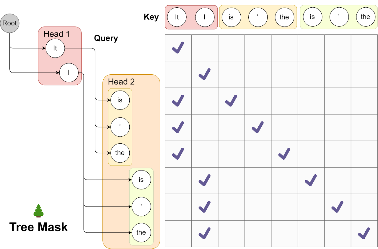
A full Cartesian product is $O(k^N)$ in the number of heads and quickly becomes unusable, so Medusa builds a fixed, sparse tree with a node budget (say 64 nodes), allocated offline: measure each head's top-$j$ accuracy on a held-out calibration set, then greedily keep the (head, rank) pairs with the highest expected acceptance. Deeper heads are less accurate, so they get fewer branches, and you end up with something like top-5 × top-2 × top-1 across the first three heads.

The tree structure pays off twice, because many paths share prefixes. Rather than flattening naively into independent candidates, shared prefixes are computed once, so a tree with hundreds of distinct root-to-leaf paths might be only 64 tokens of actual compute.

EAGLE-1: autoregressive drafting

Medusa's bet is on parallelism. All $K$ guesses are produced simultaneously from a single hidden state, which is what makes drafting nearly free, since the heads ride along on a forward pass the target was doing anyway. The cost of that bet is the missing inter-token dependency, and the deeper into the block you go the more each guess is unconditioned speculation.

EAGLE takes the opposite route: make the drafter genuinely autoregressive again, so each drafted token is conditioned on the ones before it, and pay for that conditioning as cheaply as possible. Medusa buys cheap drafting and gives up coherence within the block; EAGLE buys coherence and has to find a way not to pay full price for it. Most of what follows in this post moves along that same parallel-versus-sequential axis.

Why was autoregression expensive in the first place? In the original two-model setup, the drafter was an entire transformer run $\gamma$ times in sequence, so drafting a block of 5 meant 5 full forward passes through the small model. EAGLE's observation is that the recurrence itself was never the expensive part; running a whole transformer per step was. So keep the recurrence, shrink each step to a single decoder layer, and run that layer in feature space rather than token space.

Feature-space autoregression

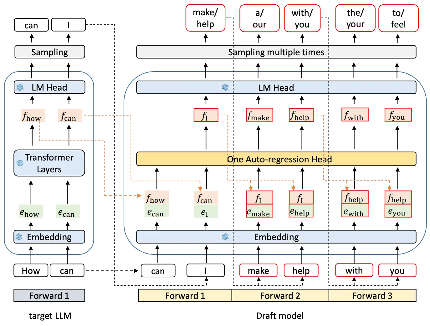
By feature we mean the same object Medusa exploited: the last hidden state, the vector just before the LM head. At each position the EAGLE draft layer consumes the feature from the previous position and the embedding of the token actually sampled there, fuses them, and predicts the next feature:

$f_{t+1} = \text{DraftLayer}\big([,e(x_{t});\ f_{t},]\big), \qquad x_{t+1} \sim \text{LMHead}(f_{t+1})$

The predicted $f_{t+1}$ lives in the same $d$-dimensional space as the target's own hidden states, so the frozen, shared LM head applies to it unchanged and no new head is trained. Sample a token from it, embed that token, feed it back alongside $f_{t+1}$, roll forward. It is a mini single-layer autoregressive model strapped on top of the target, and the loop is what supplies the inter-token dependency Medusa lacked, since step $k$ genuinely sees what step $k-1$ produced.

Why fuse the token embedding

Look again at the draft layer's input. It takes two things: the previous feature $f_t$, and the embedding of the token $x_t$ that was sampled from that feature. The first is the obvious ingredient. The second looks redundant, since $x_t$ was drawn from $f_t$ and might seem to add nothing the feature does not already carry. But it isn't redundant.

Grounding. The sampled token is a discrete, error-free anchor. At inference, from step 2 onward, the drafter consumes its own predicted features, which carry error. Feed a slightly-wrong feature back in, predict from it, and the next feature is wronger still. Without re-injecting the clean token each step, the feature trajectory drifts off-manifold within a couple of steps and the drafted tokens stop resembling anything the target would produce. The token re-grounds the trajectory every step: whatever the feature has drifted toward, the discrete token that was actually sampled is a fact, and it pins the drafter back to a real point in sequence space.

Capacity. A single decoder layer cannot reconstruct deep context from tokens alone; that is what the target's full stack is for. So hand it $f$, the target's own near-final representation, and it only has to compute the one-step delta rather than re-derive the context from scratch. The token keeps the layer honest to what a normal transformer does, since what continues forward is the token that was actually sampled, while the feature is the leapfrog that lets one layer behave like a final layer bolted onto the base model.

Prefill, decode, and trees on both sides

Because the drafter is a small transformer in its own right, it has the same prefill/decode split as any transformer. On the first pass it ingests the accepted prefix at once, the feature sequence fused with the token-embedding sequence shifted one position ahead (feature $f_i$ pairs with the token sampled from it), builds its KV cache, and only then decodes autoregressively one feature at a time. Prefix features come directly from the target's last forward pass, so they are free, and token embeddings come through the frozen embedding layer.

EAGLE keeps tree attention from Medusa, but the tree now appears on both sides. In Medusa the tree was purely a verification-side trick: generation was independent heads that never talked, so a depth-3 candidate was just three guesses stapled together and required no attention to produce. Because EAGLE drafts autoregressively, generating the tree is itself tree-structured. Branching at a node means re-running the draft layer conditioned on that node's token, so each branch's children are genuine conditional continuations of that branch, different from a sibling's children. A depth-3 EAGLE path is a coherent autoregressive continuation rather than three independent guesses, which is exactly why EAGLE accepts deeper into the tree.

Mechanically, drafting a depth-$d$ tree costs $d$ sequential draft-layer passes, one per depth level, each expanding all current leaves in parallel under a tree mask. That is the price of the sequential bet, and how many sequential draft passes a tree costs is precisely the question later methods attack.

One thing EAGLE-1 does not change: the tree shape is still static, a predetermined topology under a fixed node budget, same as Medusa. Drafting became context-aware; topology did not. We spend the same branching pattern on "2+2=" as on open-ended chat.

EAGLE-2: making the tree dynamic

EAGLE-2 addresses exactly that. How much you should branch depends on how uncertain the drafter is: after "2+2=" there is essentially one plausible continuation and branching is wasted budget, while in open chat there are many and spending nodes on alternatives pays.

So EAGLE-2 uses the drafter's own confidence to shape the tree at runtime. Draft probability turns out to be a decent proxy for eventual acceptance probability, so expand greedily toward high-confidence branches and prune low-confidence ones under a fixed node budget.

# EAGLE-2: grow the tree where the DRAFTER is confident (~ accept prob),
# instead of Medusa's offline-fixed shape.
def expand(root, budget):
    frontier = [root]
    while budget > 0 and frontier:
        node = pop_highest_confidence(frontier)   # draft prob ≈ accept prob
        for tok in node.topk_children():
            frontier.append(add_child(node, tok))
            budget -= 1

Note that dynamic trees change the shape of the tree, not the total budget. The drafter still gets exactly 64 nodes, or whatever the budget is, and only decides where to spend them. That distinction matters later, since the budget itself eventually becomes a live variable in DSpark.

Training EAGLE-1/2

The training objective deserves its own look, since it is what EAGLE-3 ends up discarding.

Conveniently, the target model manufactures its own training data. Run the frozen target over a corpus and at every position $i$ store two things: the token $t_{i+1}$ and the feature $f_i$. Now train the drafter to predict $f_{i+1}$ from $(f_i, e(t_{i+1}))$, for which the targets have already been harvested. No labelling, no separate dataset. The loss is

$L = L_{\text{reg}} + \alpha ,L_{\text{cls}}$

with a primary dense feature-regression term,

$L_{\text{reg}} = \text{SmoothL1}\big(\hat f_{i+1},\ f_{i+1}\big)$

supervising all $d$ dimensions of the vector rather than a single token, which makes learning fast, plus a small-weight token classification term that pushes both features through the frozen LM head and matches the resulting distributions:

$L_{\text{cls}} = \text{CE}\big(p_{\text{target}},\ \hat p_{\text{draft}}\big),\qquad \hat p = \text{softmax}(\text{LMHead}(\hat f_{i+1}))$

Two problems follow from this setup. The first is exposure bias: training always feeds the drafter the target's clean features, but at inference, from step 2 onward, it consumes its own predicted $\hat f$, which carries error. The drafter is never trained on the inputs it will actually see. EAGLE-1 band-aids this by adding noise to the input features during training, which helps but does not close the gap.

The second is more fundamental, which is that the objective is wrong. We do not care whether the drafter reproduces the target's features, we care whether its tokens get accepted. Feature regression is a proxy for that, and optimizing a proxy leaves performance on the table.

EAGLE-3

EAGLE-3 resolves both with a single change: stop supervising features, and train the drafter under the conditions it will face at inference. Instead of matching one-step features, the drafter is unrolled on its own generated features for several steps during training and supervised on the tokens it produces, which the paper calls a training-time test.

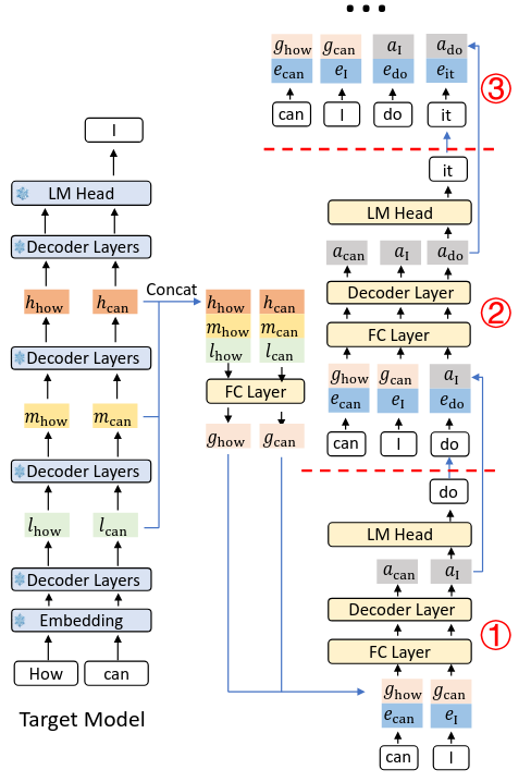
The decoding process makes the difference concrete. The input at each prefix position is a target feature paired with the embedding of the token sampled from it. These pass through a decoder layer producing an output $a$, which goes through the LM head and is sampled to obtain a draft token. In the next autoregressive step, $a$ is concatenated with that token's embedding and used to predict the next token. Mechanically this resembles EAGLE-1, but the interpretation of $a$ has changed: it is no longer trying to be the target's feature, it is simply whatever internal representation is most useful for predicting the next token. By consuming its own latent output, the drafter learns to use its own representations rather than pretending they are the target's.

Crucially, nothing forces $a$ to match the target's feature any more. The drafter is trained only to predict tokens, which is the thing we actually cared about. And since it consumes both target features at the prefix and its own outputs during the roll-forward, training includes unrolled steps where $a$ is generated and fed back so the drafter sees both input types. One such step suffices, and it eliminates the train/test gap that noise injection was papering over.

Removing the feature-matching constraint has a second consequence, and it is the one that yields most of the gain. Forcing the drafter to reproduce the target's top-layer feature is an information bottleneck, since that feature is over-specialized for the target's own next-token prediction and the deep stack has already discarded information that is irrelevant for predicting $t{+}1$ but genuinely useful for guessing further ahead. Once the drafter is no longer required to output something that lives in that space, its input is free to be anything, so EAGLE-3 feeds it a learned fusion of low, mid, and high target hidden states, combined by a linear layer. Richer semantic information in, and no error accumulation from chasing a moving feature target.

DeepSeek V3 MTP: native drafting

Everything so far has been post-hoc. You take a frozen, finished model and bolt a drafter onto it afterward, whether that is Medusa's heads or EAGLE's decoder layer. The target is never aware that speculation is happening, and the drafter's job is to reverse-engineer a model that was trained with no thought of being drafted for.

Multi-Token Prediction, introduced at frontier scale in DeepSeek-V3, asks what happens if you stop treating speculation as an afterthought. The draft modules exist during pretraining and are trained jointly with the main model, so the target learns alongside them.

Architecture

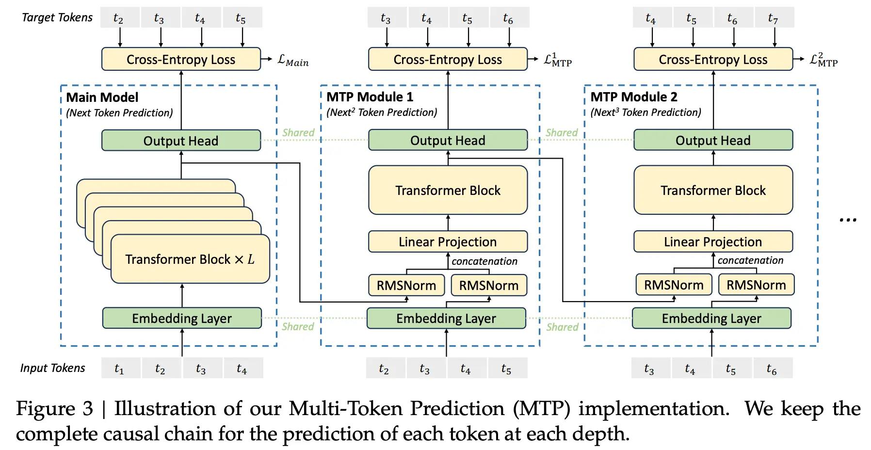
MTP predicts $D$ extra tokens using $D$ sequential modules chained one after another. Module 1 is nearly an EAGLE step living inside the model: take the main model's top-layer feature, pair it with the embedding of the token that feature produced, project to a shared space, run a transformer block, read out through the shared head.

Concretely, module $k$ at position $i$ fuses $h_i^{k-1}$ with $e(t_{i+k})$ and predicts $t_{i+k+1}$. That indexing is dense, so take the simplest case, the first position and first module ($i=1$, $k=1$). The input feature $h_1^0$ is the main model's top-layer hidden at position 1, the vector passed through the LM head to predict $t_2$. Pair it with $e(t_2)$, the embedding of the token that feature actually produced, and train the module to predict $t_3$.

The pattern is the one EAGLE established. The feature is a compression of all the computation the main model did to predict the next token, so handing the module that vector plus the token chosen from it leaves only the small delta for the token after, and the digested context comes for free.

The chain

Chaining several modules is where MTP diverges from EAGLE, in a way that is easy to misread.

EAGLE reuses a single draft layer, calling it repeatedly and feeding its own sampled-token embedding back in. MTP reuses nothing: the modules are distinct per depth, each with its own projection $M_k$ and its own transformer block $\text{TRM}_k$. Depth 2 is a different set of weights from depth 1, trained specifically for the job of predicting two tokens out.

What gets passed along the chain also differs. Module 2 does not receive the main model's feature. It receives module 1's output hidden $h_i^1$, at the same position $i$, pairs it with $e(t_{i+2})$, and predicts $t_{i+3}$. So the hidden state is what chains forward, and it stays at a fixed position, while the token embedding being injected advances by one at each depth.

The two axes move independently, which is the clearest way to hold the picture: the hidden marches down the depth axis at a frozen position ($h_i^0 \to h_i^1 \to h_i^2$) while the injected token embedding marches along the sequence axis ($t_{i+1}, t_{i+2}, t_{i+3}$), and each depth consumes the next real token and predicts the one after. During training that injected token is the teacher-forced ground truth; at inference it is the token the previous module produced, but the pairing is identical either way.

Loss

Each depth contributes an auxiliary cross-entropy loss for its own target token, added to the main language modeling objective. Because the modules train alongside the main model, gradients flow back into the shared trunk, which forces every hidden state to encode information about several future tokens rather than just the next one.

This is where MTP earns its keep twice over. DeepSeek report that the auxiliary objective raises the main model's benchmark scores, so the machinery that enables speculation also improves the model doing the speculating. There is also no train/test gap by construction, since the modules were never trained on inputs different from the ones they see at inference.

In later papers you will see this reported as MTP-1, meaning one module speculating one token ahead. It is worth registering, because it is the production baseline DSpark is measured against.

DFlash: returning to parallel drafting

By this point the field has explored both directions fairly thoroughly. EAGLE and MTP draft sequentially, so a length-$\gamma$ block costs $\gamma$ drafter runs and $T_{\text{draft}} \propto \gamma$, which buys inter-token dependency and high acceptance. Medusa made the opposite bet, all $\gamma$ tokens in one pass with $T_{\text{draft}}$ roughly constant in $\gamma$, but no inter-token dependency and therefore acceptance that collapses down the block.

Sequential drafting won that argument, and for a while the parallel branch looked like a dead end. But the reason Medusa failed is more specific than parallel drafting not working. Medusa's heads failed because they were independent, each producing its own marginal over its own position with no mechanism for the positions to coordinate. Parallelism was not the problem; independence was.

That distinction leaves an opening. Generate all $\gamma$ positions in one pass while still letting them condition on each other, and you get Medusa's latency with something closer to EAGLE's coherence. There is an existing family of models built to do exactly that.

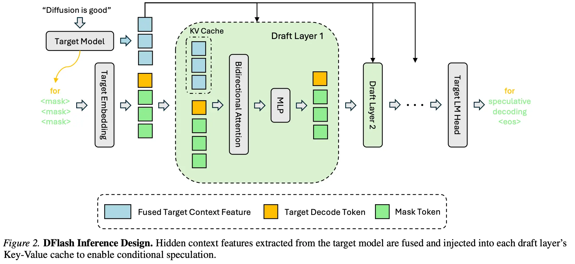
Borrowing from diffusion language models

Diffusion language models generate by masking and unmasking rather than left to right. The relevant variant here is block diffusion, which handles text one block at a time: lay out a block of masked positions, then fill them in simultaneously, with bidirectional attention so that every position can see every other. That last part is the key difference from Medusa, whose heads were blind to each other. A bidirectional block is not. The positions are still resolved in one pass, but they are resolved jointly, as a coordinated set rather than as independent guesses.

Diffusion LMs have a known weakness, which is that they tend to underperform autoregressive models on generation quality. In a standalone generator that is disqualifying. In a drafter it matters much less, because quality is the verifier's job, and per the guarantee established at the top of this post the output distribution is unchanged no matter how mediocre the drafter is. A drafter is allowed to be wrong. It is only not allowed to be slow.

DFlash exploits precisely that division of labor: diffusion for fast parallel drafting, autoregression for high-quality verification. The drafter is a block diffusion model conditioned on the target's hidden states, filling a whole block of draft tokens in a single forward pass.

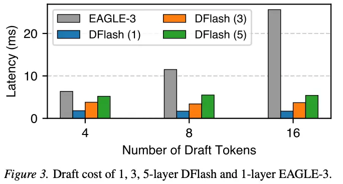
The payoff goes beyond the obvious latency win. Because drafting cost is now roughly constant in $\gamma$ rather than proportional to it, a diffusion drafter can afford deeper, more expressive architectures and still be faster than a shallow autoregressive drafter, and the ablations below suggest that is where the gains actually come from. The following figure depicts a latency comparison between DFlash at different layer depths and EAGLE-3.

Diffusion beating autoregression??

The headline result has DFlash roughly doubling acceptance length over EAGLE-3:

Q3-4B, T=0, avg $\tau$	EAGLE-3 (tree 16)	EAGLE-3 (tree 60)	DFlash (block 16)
$\tau$	3.05	3.48	6.54

Autoregressive transformers are the uncontested frontier in language modeling, so how is a diffusion drafter aligning better with the target? It is not, and the ablations say so plainly. Isolating the drafting paradigm with everything else held fixed:

Conditioning	GSM8K	HumanEval	MT-Bench
AR drafting (DFlash-AR)	KV inject	4.8 / 2.4x	4.6 / 2.3x
Diffusion drafting (DFlash)	KV inject	4.2 / 3.3x	4.0 / 3.2x

Pound for pound, with depth, block size, target features, and conditioning all fixed, autoregressive drafting still wins on $\tau$. Diffusion loses on acceptance and wins on speedup, which is the $T_{\text{draft}}/\tau$ trade-off doing its work.

The headline gains therefore come from depth. Autoregressive drafters are forced to stay shallow because each pass is repeated $\gamma$ times, so every layer is paid for $\gamma$ times over, whereas DFlash pays for depth once and spends the savings on the axis that actually buys acceptance length. Acceptance grows monotonically with layer count, and DFlash can afford a 5-layer drafter where EAGLE cannot.

Three ingredients keep it from repeating Medusa's failure:

1. Intra-block dependency via bidirectional attention. Block diffusion denoises all positions in one pass, but the positions attend to each other. This is not causal autoregressive dependency, it is joint prediction, and isolated it sits only about 0.5 tokens behind AR on acceptance length.
2. Target-feature conditioning. Conditioning on the target's hidden states, rather than training a standalone diffusion drafter as earlier diffusion-based speculative methods did. The target's features implicitly carry information about tokens beyond the immediate next one, which is the recurring free lunch of this whole literature.
3. KV injection. Injecting target features as KV states lets every drafter layer attend to them directly, instead of feeding them only as initial input where their content dilutes with depth. Not diffusion-specific; it helps AR too.

But what is "block diffusion"?

The term has been doing a lot of work above, so here is what it amounts to mechanically. When DFlash drafts, it lays out a fixed-size block and fills it in one pass:

[ anchor ] [ MASK ] [ MASK ] [ MASK ] ...
   clean       ← predict these B-1 in one pass →

A [MASK] is a special token meaning "something goes here, figure out what", a mask embedding plus positional information, carrying no content of its own. The block goes through the draft stack once with bidirectional attention, so every mask sees every other position, and a token distribution is read out at each masked slot.

The anchor comes free. Every verification cycle the target commits at least one guaranteed-correct token, the bonus token, and it becomes the clean anchor at the front of the next block. The drafter's situation is always identical: given one known-good token, predict the run that follows.

Training is BERT-style masked language modeling with a twist: corrupt a sequence by replacing tokens with [MASK], ask the model to reconstruct them, but let the mask ratio vary all the way from none to everything. Generation runs this backward, starting from a fully masked span, predicting, keeping the confident tokens, re-predicting the rest, and repeating.

That iterative loop exists for a reason. Filling every mask in one pass produces each position's prediction independently, since no mask sees what its neighbors actually turned into, only that they are masks, which is the Medusa problem restated. Full diffusion LMs buy coordination back by taking many denoising steps with re-conditioning in between, and that is also why they are slow, need a fixed-length canvas, and cannot reuse a KV cache, since any position can change on any step.

Block diffusion is the middle ground: autoregressive across blocks, diffusion within a block. Think of block size as a dial, where size 1 is plain autoregression and block-equals-whole-sequence is full diffusion. In between you get within-block parallelism while keeping the two things full diffusion throws away, variable length (emit blocks until EOS) and a usable KV cache (finished blocks freeze, so later blocks reuse them). That across-block rhythm is exactly a drafter's rhythm, draft a block, verify, advance, which is why block diffusion slots into the speculative decoding framework so naturally.

DFlash then takes the aggressive extreme, one denoising step per block. No re-conditioning, no iterative refinement, fully masked block in, all tokens out. This is what keeps drafting cheap regardless of block length, and what earns the "flash". In the end DFlash's diffusion is really the training recipe plus the bidirectional block, since the iterative diffusive trajectory is gone.

And that trajectory was the thing buying coordination between positions. Bidirectional attention recovers some of it, since the masks at least attend to each other, but each position's final token is still sampled from its own marginal without seeing what its neighbors resolved to.

DSpark

That gap is where DSpark starts. It takes DFlash as its backbone and addresses the fact that drafted positions are generated jointly but each token is still ultimately drawn from its own marginal, without conditioning on what the positions before it actually resolved to.

Both poles are clear by now. Autoregressive drafters get strong acceptance by conditioning each token on the ones sampled before it, but pay $T_{\text{draft}} \propto \gamma$, which forces them shallow. Parallel drafters collapse drafting to a single pass so $T_{\text{draft}}$ is near-constant in $\gamma$, allowing real depth, but predict each position independently and decay fast down the block. Both bets have a clear downside, and the field has spent several years alternating between them.

DSpark's move is to stop choosing. Keep the fast parallel backbone for the heavy lifting, then bolt on a cheap sequential stage that reintroduces inter-token dependency without reintroducing the $O(\gamma)$ cost. The result is semi-autoregressive: parallel where parallelism is affordable, sequential where sequence actually matters.

Semi-autoregressive architecture

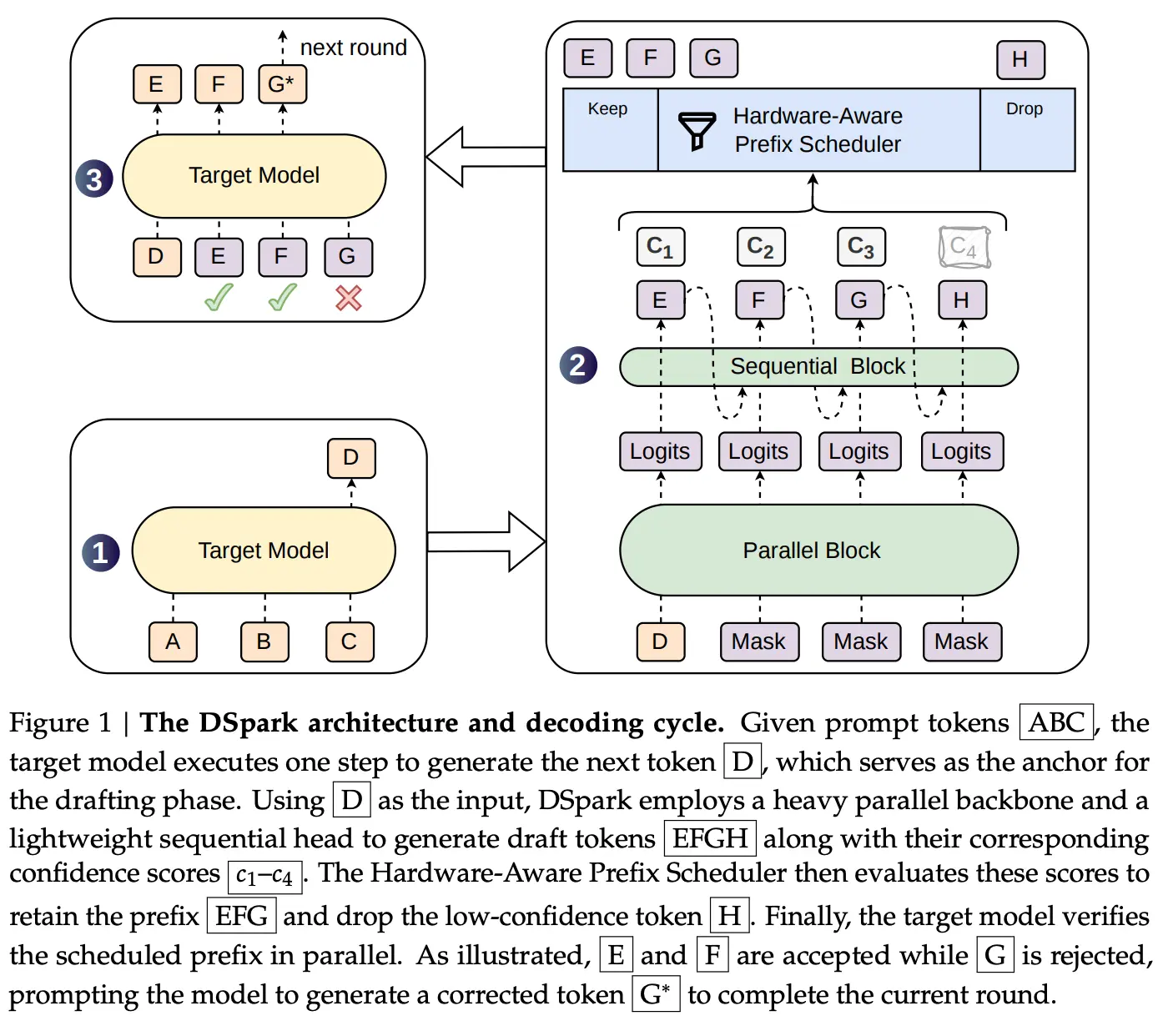
Parallel stage. The backbone is DFlash, essentially unchanged. One bidirectional pass over the block produces hidden states $h_1, \dots, h_\gamma$ and base logits $U_1, \dots, U_\gamma$. This is the expensive, context-rich part, and it is where the depth advantage lives. But exactly as in DFlash, $U_k$ is a marginal preference, since it never saw what was sampled at the other positions because they were masks. It captures what kind of token belongs at position $k$, not coherence with its actual neighbors. That missing coherence is the suffix-decay problem, and repairing it is the sequential stage's only job.

Sequential stage. The sequential stage adds a prefix-dependent transition bias $B_k$ to the base logits, letting each position finally condition on the tokens actually sampled before it. The obvious way to do this would be to define a joint energy over the whole block, but that requires a partition function summing over $V^\gamma$ possible blocks, which is hopeless. Instead DSpark induces a proper causal block distribution by autoregressive factorization:

$P(X \mid x_0) = \prod_{k=1}^{\gamma} p_k(x_k \mid x_0, x_{<k}), \qquad p_k(v \mid x_0, x_{<k}) = \frac{\exp!\big(U_k(v) + B_k(x_0, x_{<k}, v)\big)}{\sum_{u \in \mathcal{V}} \exp!\big(U_k(u) + B_k(x_0, x_{<k}, u)\big)}$

Read the logit as two added terms. $U_k(v)$ is the base logit from the parallel backbone, computed once, independent of $x_{<k}$. $B_k$ is the correction that does depend on previously sampled tokens and the anchor $x_0$. Each position is locally normalized over the vocabulary, and the chain rule stitches the local softmaxes into a valid joint. Tractable, and a proper distribution, which matters because verification needs a well-defined $q$ to compute acceptance probabilities against.

The bias is additive on purpose. The backbone already did the expensive contextual work inside $U_k$, so the head only computes the one-step delta: given that position $k{-}1$ actually resolved to of, push toward course, suppress problem. That is what lets the head be tiny, and tiny is mandatory, because the sequential loop runs $\gamma$ times in series. We need $T_{\text{sequential}} \ll T_{\text{parallel}}$ or the parallel advantage evaporates and we are back to EAGLE's cost structure.

Two instantiations, differing only in how much history $B_k$ sees:

Markov head. Condition only on the immediately preceding token $x_{k-1}$, a first-order dependency. A full first-order bias would be a $V \times V$ matrix, absurd at vocabulary scale, so it is low-rank factored as $B = W_1 W_2$ with $W_1 \in \mathbb{R}^{V \times r}$, $W_2 \in \mathbb{R}^{r \times V}$, $r = 256$:

$B(x_{k-1}, \cdot) = W_1[x_{k-1}], W_2 \in \mathbb{R}^V$

$W_1[x_{k-1}]$ looks up an $r$-dimensional embedding of the just-sampled token, and $W_2$ projects it to a bias over the whole vocabulary. One lookup plus one $r \times V$ matmul per step, which is nothing next to a transformer layer.

RNN head. The Markov head is memoryless beyond one step. The RNN head carries a recurrent state $s_k \in \mathbb{R}^r$ accumulating the full within-block prefix. It concatenates previous state, previous-token embedding (reusing $W_1$), and backbone hidden into $z_k = [s_{k-1};, W_1[x_{k-1}];, h_k] \in \mathbb{R}^{2r+d}$, then applies a GRU-style gated update:

$s_k = \sigma(W_g z_k) \odot s_{k-1} + \big(1 - \sigma(W_g z_k)\big) \odot \tanh(W_c z_k), \qquad B_k(x_{<k}, \cdot) = W_2^\top \tanh(W_o z_k)$

Slightly more capacity for longer intra-block dependencies, still cheap.

Why the hybrid wins

The headline numbers have both parallel (DFlash) and semi-autoregressive (DSpark) beating fully autoregressive EAGLE-3 on accepted length:

Qwen3 14B

Drafter	Math Avg.	Code Avg.	Chat Avg.
EAGLE-3	4.52	3.99	2.52
DFlash	4.74	4.45	2.92
DSpark	5.63	5.24	3.47

Gemma4 12B

Drafter	Math Avg.	Code Avg.	Chat Avg.
EAGLE-3	5.39	4.75	2.99
DFlash	4.90	4.35	2.80
DSpark	5.65	5.09	3.25

As the authors note, this contrasts with the standard expectation that step-by-step autoregression produces higher-quality sequences than parallel models. Their per-position acceptance analysis explains it, and it is the most illuminating result in the paper.

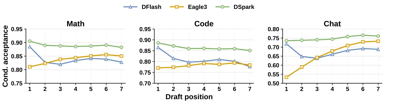
At the first draft position, DFlash and DSpark substantially outperform EAGLE-3. This is the architectural capacity argument again, with autoregressive drafters constrained to be shallow by their $O(\gamma)$ latency while parallel drafters can afford depth. And because speculative decoding is a strict prefix-matching survival process, the first token carries the highest leverage, since a rejection there invalidates the entire block immediately no matter how good the rest of the guesses were. An early-position capacity advantage therefore propagates disproportionately into final accepted length.

At the tail, the picture inverts. Once tokens are locked into a semantic path, subsequent tokens become more predictable, and autoregressive models exploit this: EAGLE-3 maintains or even increases acceptance deeper into the block. DFlash decays hard, because independent parallel generation has nothing to exploit.

DSpark inherits both, taking high early acceptance from the deep parallel backbone and stable acceptance deep into the block from the sequential head.

The gains scale with proposal length, exactly as that reading predicts. DSpark and DFlash are roughly equal below 4 tokens, where there is little suffix for the sequential head to fix, then DSpark pulls ahead by about 17% at $\gamma = 7$ and about 25% at $\gamma = 15$. And the cost is almost nothing, with proposal length scaling from 4 to 16 adding between 0.2% and 1.3% latency overhead despite the sequential stage. A very small amount of autoregression goes a long way.

Verify smarter, not longer

So DSpark can produce long, high-quality draft blocks cheaply, and the natural conclusion would be to always draft and verify as much as possible. In production that conclusion is wrong, and prior work barely discusses why.

Producing more draft tokens does not automatically translate into end-to-end speedup, because verification is not free: every draft token occupies a slot in the target model's forward pass. In a lightly loaded system that compute is effectively free, since there is headroom in the batch and the accelerator is underutilized anyway. In a large-scale serving system with constant incoming requests it is not, and filling batch capacity with verification tokens that end up rejected is wasted work that could have served other requests. With many concurrent requests each contributing draft tokens per forward pass, this becomes a resource allocation problem: how much compute should go to verification, and which draft tokens are worth it.

DSpark's answer starts with a confidence head that emits a scalar in $(0,1)$ per draft position, an estimate of whether that token will survive verification. Sweeping a static confidence threshold over this is instructive. A threshold of zero recovers standard fixed-length verification, as in every prior method. As the threshold rises, overall acceptance rate climbs, confirming the estimator genuinely identifies tokens that would have been rejected, and higher acceptance means less wasted work.

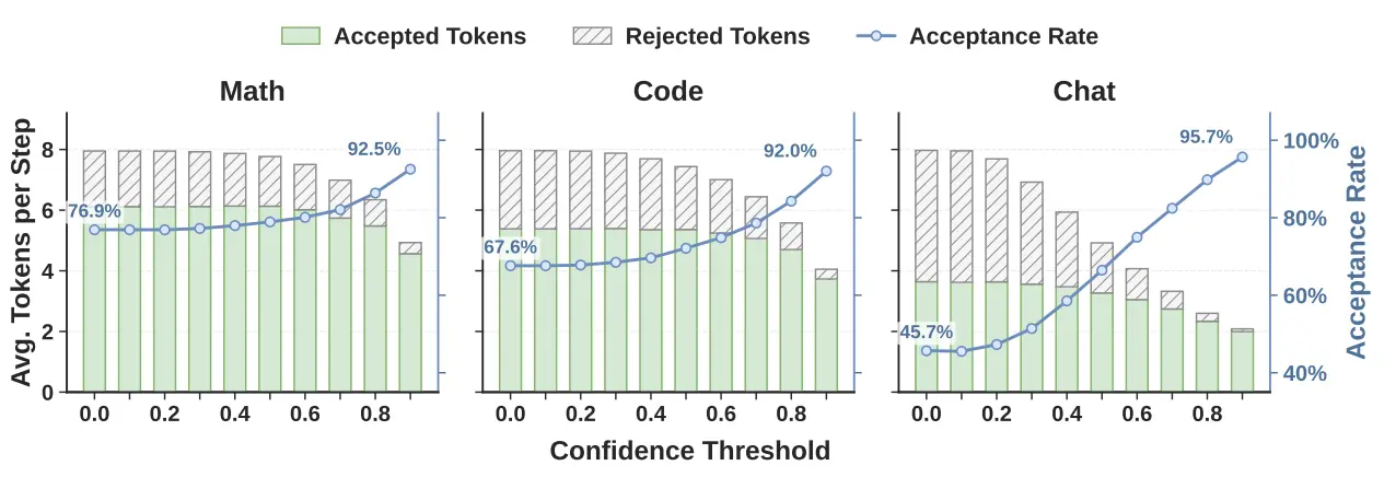
But no single static threshold is right. Raising it also discards tokens that would have been accepted, and the behavior differs by domain. In chat, raising the threshold immediately prunes a large number of tokens, while in math and code pruning is milder and more tokens survive. Chat is inherently higher entropy with fewer obvious continuations, so the drafter guesses more, and via the confidence head it knows it is guessing more.

The static threshold is a useful diagnostic, but the real conclusion is that proposal length should be a dynamic function of system load: verifying low-confidence tokens incurs minimal opportunity cost under low concurrency, but wastes critical batch capacity under high concurrency. Hence a hardware-aware prefix scheduler, wrapping the inference engine, which schedules draft tokens into the next forward pass based on current load and per-token confidence. Note what has happened to the node budget along the way: fixed and offline in Medusa, fixed with dynamic shape in EAGLE-2, and now a live variable set per step by the serving system.

DSpark in a production environment

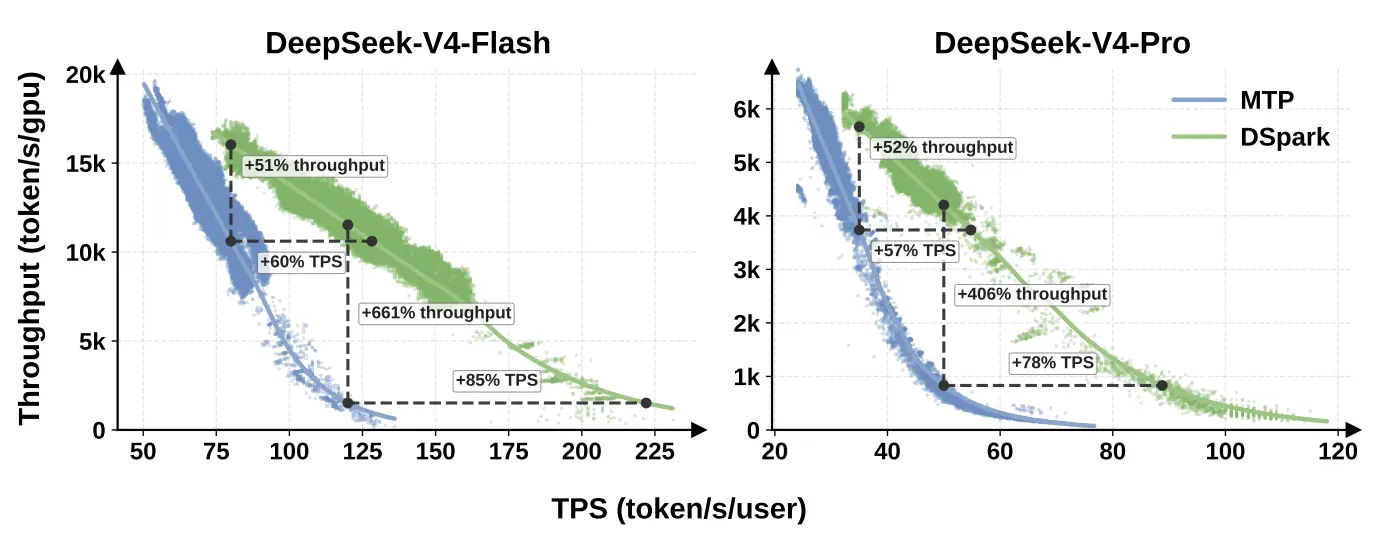
Production serving has a standard throughput/interactivity trade-off. At low concurrency, few requests are processed per decoding step, so per-user generation speed is high but aggregate GPU throughput is low, since weight movement is poorly amortized and the accelerator is underutilized. As concurrency increases, effective batch size grows and total tokens/s/GPU improves, but each request progresses more slowly.

In DSpark's deployment, concurrency is typically capped by KV-cache capacity or available user traffic before the GPU reaches compute saturation. With active requests fixed, aggregate throughput and per-user speed become aligned:

$\text{tok/s/user} \approx \frac{\text{total tok/s/GPU}}{\text{active requests}}$

The significance of running below saturation is not that it creates this relationship, but that it leaves unused compute that can be converted into progress for existing requests.

DSpark spends that headroom on speculative verification. The drafter cheaply produces a longer block, up to $\gamma = 5$, and the scheduler ranks candidate prefix extensions by cumulative survival probability. Under light or moderate load it verifies more high-confidence tokens, raising expected accepted tokens per target step at little added latency. It does not simply maximize verification length; it adds tokens only while their expected benefit outweighs the reduction in steps per second caused by the larger verification batch.

MTP-1, fixed at one draft token, cannot exploit spare capacity at all. DSpark therefore moves the throughput/interactivity frontier by adapting its verification budget to load, spending otherwise-idle compute when capacity exists and then shortening verification as concurrency rises so speculative work does not consume batch capacity that real requests need. The effect is largest exactly where the headroom is, at low concurrency. Under a strict 120 tok/s/user requirement, DSpark achieves 661% higher aggregate throughput for DSV4 Flash.

References

• Medusa: Simple LLM Inference Acceleration Framework with Multiple Decoding Heads
• EAGLE: Speculative Sampling Requires Rethinking Feature Uncertainty
• EAGLE-2: Faster Inference of Language Models with Dynamic Draft Trees
• EAGLE-3: Scaling up Inference Acceleration of Large Language Models via Training-Time Test
• DeepSeek-V3 Technical Report
• DFlash
• DSpark