State of FP8 Training + K2 INT4

November 13, 2025.

FP8 training is notoriously ambiguous—honestly, quantization in general is fuzzy because there are so many distinct components in a training or inference pipeline that can be quantized. I wanted to drill down into exactly what we mean by FP8 Training, because for a long time I operated under the assumption that this implied most, if not all, components were cast in FP8. Turns out, that's far from the case. What follows is a brief overview of the history of FP8 training, leading up to DeepSeek-V3 (DSV3)—arguably the standout success story in FP8 training so far—and concluding with more recent attempts from the Ling Team. I might turn this into a proper blog post at some point, the content is all here but it needs to be polished, right now its just notes I took while reading.

Data format	Max normal	Min normal	Min subnormal	Maximum Relative Error (Min - Max)
FP32 (S1E8M23)	3.40 × 10³⁸	1.18 × 10⁻³⁸	1.40 × 10⁻⁴⁵	1.19 × 10⁻⁷ ∼ 5.96 × 10⁻⁸
FP16 (S1E5M10)	65,504	6.10 × 10⁻⁵	5.96 × 10⁻⁸	9.76 × 10⁻⁴ ∼ 4.89 × 10⁻⁴
BF16 (S1E8M7)	3.39 × 10³⁸	1.18 × 10⁻³⁸	9.18 × 10⁻⁴¹	7.75 × 10⁻³ ∼ 3.94 × 10⁻³
FP8 (S1E4M3)	448	1.56 × 10⁻²	1.95 × 10⁻³	1.11 × 10⁻¹ ∼ 7.69 × 10⁻²
FP8 (S1E5M2)	57,344	6.10 × 10⁻⁵	1.53 × 10⁻⁵	2.00 × 10⁻¹ ∼ 1.67 × 10⁻¹

NVIDIA released the H100 GPU back in late 2022, which offered support for FP8. In theory FP8 could achieve substantial speed ups but the current landscape provided no support for proper FP8 training. As described in the FP8-LLM paper "Unfortunately, the current support for FP8 training is rare and limited. The only usable framework is the Nvidia Transformer Engine (TE), but it applies FP8 solely for GEMM computation and still retains master weights and gradients using high precision, e.g., FP16 or FP32." This means that only the matrix multiply-accumulate in the linear/attention projections is executed with FP8 operands on Tensor Cores, while everything else (LayerNorm, softmax, residual adds, loss/optimizer math) and the model state you keep around (master weights, optimizer states, and usually saved activations for backward) stays in higher precision (BF16/FP16/FP32). NVIDIA’s Transformer Engine (TE) exposes this via fp8_autocast around modules like Linear; inside that region, TE casts the GEMM operands to FP8 and tracks the per-tensor scaling.

FP8 GEMM

The FP8 GEMM introduced in Hopper enables FP8 computation in the Tensor Core. This can be done either via directly injecting FP8 input, or through casting of higher precision input on the fly. In the lower-level language, you specify input types, compute type and scaling modes.

Choose/refresh scales (per tensor/row/col or block)
TE maintains an amax history and computes a scale s for each FP8 tensor (e.g., s_x for X, s_w for W). “Delayed scaling” uses the previous iterations’ maxima so you don’t need a second pass.
On-the-fly quantization of operands
Right before the matmul, TE casts working copies of X and W from BF16/FP16 to FP8 using those scales, producing X8 = Q(X / s_x) and W8 = Q(W / s_w). TE’s own primer spells this out: in FP8 execution “both the input and weights are cast to FP8 before the computation.”
cuBLASLt matmul with FP8 inputs, higher-precision math
The GEMM runs with FP8 A/B, compute type = FP32, and an FP16/BF16/FP32 D. cuBLASLt applies the configured scaling inside the kernel (tensorwide / outer-vector / 128-elem or 128×128 block), effectively computing
$D_{ij}=s_A\cdot s_B\cdot \sum_\ell \widehat{X_8}_{i\ell}\widehat{W_8}_{\ell j}.$
Epilogue + output precision
The accumulator Y_acc is written out in your chosen storage type—commonly BF16/FP16 for training state, or sometimes re-quantized to FP8 (with its own output scale s_y) if you’re aggressively minimizing bandwidth between layers. (TE exposes these choices; it also updates the amax stats for the next iteration)

So even if master weights and gradients are kept in FP16/FP32, the compute path does: BF16/FP16 → FP8 (with scale) → GEMM (FP32 accum) → BF16/FP16 (or FP8) output.

Scale Factor

The key technique behind overcoming the challenges of low-precision training associated with representation range and precision degredation is tensor scaling. Tensor scaling scales the tensor values that originally locate out the representation range of a data format to its comfort zone

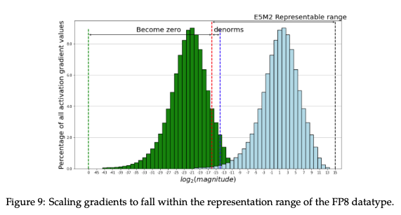
The pioneer scaling techniques apply a global scaling factor to the loss, such that gradients of all layers are scaled by a single adaptive factor. The utilization of the global loss scaling technique, has facilitated the widespread adoption of FP16 mixed-precision training on V100 and A100s. Gradients are especially susceptible to underflow in representations with a low dynamic range (such as FP16), training in BF16 (same dynamic range as FP32) does not suffer from this problem, meaning it doesn't require a loss scaling, and has therefore been standard in LLM training for quite some time.

While the dynamic range provided by the FP8 types is sufficient to store any particular activation or gradient, it is not sufficient for all of them at the same time. This makes the single loss scaling factor strategy, which worked for FP16, infeasible for FP8 training and instead requires using distinct scaling factors for each FP8 tensor: tensor scaling. There are two types of tensor scaling:

Just-in-time. This strategy involves determining the scale factor based on the amax of the tensor being generated. However, in practical applications, this approach is infeasible because it necessitates multiple passes through the data. Specifically, the operator first produces and writes out the output in higher precision, then calculates the maximum absolute value of the output, and finally applies this scaling factor to all values to obtain the final FP8 output. This process introduces a significant amount of overhead, which can substantially reduce the benefits of using FP8.
Delayed. This strategy involves selecting the scaling factor based on the maximum absolute values observed in a certain number of preceding iterations. This approach allows for the full performance benefits of FP8 computation but necessitates the storage of a history of maximum values as additional parameters of the FP8 operators.

Note on Delayed vs JIT: It may not be immediately obvious why JIT is slower than Delayed, considering both strategies require calculating the amax of the tensor (JIT needs it to perform the quantization and Delayed needs it for the next iteration quantization). Consider a BF16 tensor $X$ , in JIT we calculate $s = \frac{\text{FP8\_MAX}}{\max(|x|)}$ to quantize the tensor, requiring a reduction over the tensor. In Delayed, we already have $s$ from our history, meaning that we can directly quantize $X$ , but what about the amax required for future iterations? Well there is a very nice fused operation we can use that quantizes $X$ and spits out the amax at the same time. This means we can avoid the extra pre-pass to calculate amax! Something similar happens in the FP8 GEMM: Consider $C = XW$ . In a FP8 GEMM we accumulate in a higher precision for each output element $c_{ij}$ , and then cast to FP8. With JIT, we have to materialize the entire output matrix C before we can calculate amax(C) that is required to quantize the tensor. In Delayed, we can again cleverly combine these two operations, after accumulation, we can immediately cast each tile to FP8 as long as we just make sure to bookkeep a running amax. We benefit from the fact that our current scaling factor does not depend on our current amax, there is no sequential dependency between quantizing the tensor and calculating the tensors amax.

Naturally, once we've entered the space of tensor scaling, we can go beyond a tensor-wise scale factor into sub-tensor scale factors termed block scaling. The core principle behind FP8 block scaling is to enhance precision by adapting the scaling factor to localized data characteristics. Unlike per-tensor methods that apply a single scale across an entire tensor, block scaling divides each tensor into smaller, distinct segments. Within each of these defined blocks, all values share a common scaling factor stored separately in FP32 for accuracy.

FP8-LM: Training FP8 Large Language Models

While FP8 computation is faster, this single optimization is not enough to unlock nearly the true potential of FP8.

During training, memory is consumed primarily by our optimizer state, gradients and weights. The common setup under Adam is:

Setup	Param	Grad	$m$	$v$	Bytes per parameter
BF16 params, FP32 adam (common)	BF16 (2)	BF16 (2)	FP32 (4)	FP32 (4)	2 + 2 + 4 + 4 = 12 B
FP32 (AMP classic)	FP32 (4)	FP32 (4)	FP32 (4)	FP32 (4)	(2+4) + 2 + 4 + 4 = 16 B

where the remaining memory is consumed by activations, temporary buffers and unsuable fragmented memory. Of these, activations can grow in memory in transformers under very large context lengths but it does not define the typical scenario.

Ideally, you'd want to reduce the precision of all of these states. The paper starts by looking at gradients, and introduce methods to realize storing and communicating gradients in FP8. They find that directly applying FP8 to gradients leads to a decrease in accuracy, and find that this degredation stems from underflow/overflow during low-bit all-reduce. They introduce an automatic scaling technique to mitigate this. Additionally, they introduce a technique to manage the tensor-wise scaling factors associated with each gradien tensor. Fixing these issues with all-reduce they find that gradients can be stored in FP8.

Next, they look at the optimizer, and look at each part of the optimizer, trying to identify the minimal precision they can use for each component, finding that they can reduce to the following:

Setup	Param	Grad	$m$	$v$	Bytes per parameter
FP8-LM	FP16 (2)	FP8 (1)	FP8 (1)	FP16 (2)	= 6 B

Through training experiments they validate this selection, finding that is performs on par with higher-precision alternatives. Ablations find compute FP8 GEMM is stable across a bunch of settings, the same goes for FP8 comms. Master weights however are unstable under FP8 and require either FP16 with tensor-scaling or BF16. For optimizer states, the first order momentum can be reduced to FP8, while the second order needs to be stored in FP16.

Scaling FP8 Training To Trillion-Token LLMs

A follow up paper to the above, but scaling beyond just 100B tokens into the trillions. Crucially, this paper observed that outliers occur at much higher frequency as we go beyond 100B tokens, arguing that the proposed method above is not stable at real-world scales.

The authors identify the source of this issue to be the SwiGLU layers. They show that the weight vectors of SwiGLU tend to align which causes the SwiGLU output magnitude to increase significantly during training, potentially resulting in outliers. This relationship is empirically confirmed during training. At about 200B tokens, FP8 loss starts to converge, and at the same time we see that SwiGLU weight norm spikes, with their weights exhibiting high correlation when compared to early stages of training. Interestingly, the authors observe that disabling the quantization of the last linear layer in the MLP component (output of SwiGLU), allows Llama 2 FP8 to successfully converge with large datasets, let's take a closer look at how that modification looks

Disable last quantization in SwiGLU

A SwiGLU MLP (biases omitted for clarity). Let $x$ be BF16, $W_{1,8},W_{2,8},W_{3,8}$ be FP8 with scales $s_x,s_{w1},s_{w2},s_{w3}$ . Let $\widehat{\cdot}$ decode FP8 codes to real values (before scaling).

Up projections (FP8 GEMMs, FP32 accum):

X_8 = Q(x/s_x),\quad A = (s_x s_{w1})\widehat{X_8}\widehat{W_{1,8}},\quad B = (s_x s_{w2})\widehat{X_8}\widehat{W_{2,8}},

with the GEMM math accumulating in FP32; the library returns (A,B) in BF16/FP16. Non-safe operations (e.g Swish, elementwise gates, norms) are typically left in higher precision. After performing the up-projections in FP8, we perform the SwiGLU in higher precision

h = A\odot \operatorname{Swish}(B) \quad \text{(BF16/FP16)}.

The output projection is typically performed with a FP8 GEMM. Which would look like this

H_8 = Q(h/s_h),\qquad z = (s_h s_{w3})\widehat{H_8},\widehat{W_{3,8}}\quad\text{(FP32 accum)},

and return the desired outcome type (BF16). This last step is what was disabled in the aforementioned experiment, resulting in stable FP8 training. The SwiGLU operation has a tendency creating outliers as training progresses, when these outliers (found in $h$ ) are quantized prior to output-projection they introduce significant quantization errors which destabilizes training. By disabling this quantization step, we avoid such errors and allow tensors to normalize before subsequent quantization in later layers.

To address the observed issue of channel-wise outliers in $h$ , the authors introduce a slight modification to the SwiGLU output

h = s \odot (A\odot \operatorname{Swish}(B)) \quad \text{(BF16/FP16)}.

where $s$ is a scaling factor matrix that is computed from the per-channel amax over a channel on. To be clear, this rescales the BF16 activation channel-wise before the FP8 quantization that feeds $W_3$ . Think of $s$ as an extra amplitude scaling to make the pre- $W_3$ activation quantizable in FP8. After the final FP8 GEMM, we undo the scaling through $s^{-1}$ .

Peng et al (2023) found that they could reduce the first moment to FP8, but had to keep the second moment in FP16 in order to avoid training collapse. In this paper, the authors find that they are able to quantize both moments to FP8 through proper quantization schemes. The second moment in adam is an estimate of the uncentered variance of the gradients. The adam update rule uses the inverse square root of the second moment in its parameter step, naturally, such an operation means that the smallest values become the most significant in determining the parameter updates. This characteristic creates a unique challenge when considering precision reduction. The authors of this paper realize that by using E5M2 for the second moment, they have enough dynamic range to capture the necessary information about the smallest values in the second moment which are most important for the update. The additional exponent bit ensures that they can accurately represent both very small and moderately large values, which is critical given the inverse square root operation applied to this moment.

Through these techniques that are able to train stable for up to 2T tokens, compared to FP8 baselines that fail. Note: the FP8 baseline was trained using the standard format (Micikevicus et al 2022) which includes saving a high precision weight matrix and quantization to E4M3 in the forward pass and E5M2 for the backward pass with delayed scaling (similar to Nvidia Transformer Engine).

Towards Fully FP8 GEMM LLM Training at Scale

Published in spring 2025. Existing literature has proposed FP8 recipes by employing multiple scaling factors per tensor (DeepSeek V3), i.e block-scaling. However this comes with efficiency overhead, diminishing large potential gains of FP8. Other work has proposed adjusting the SwiGLU-based transformer to prevent outliers. Despite progress we are far from achieving full FP8 training, existing work focus on FP8 GEMMs within the linear projections of the transformer, maintaining higher precision for other GEMMs, namely those involved in the dot product attention mechanism. This however isn't as costly as it sounds given that linear projection FLOPs dominate attention FLOPs at reasonable context lengths (<16k). For a standard non-MoE transformer, the fractional cost of attention to other matmuls is T/8D, where T is context length and D the hidden dimension. This means that dot-product attention FLOPs only become dominant once T>8D. With D typically in the thousands, you get the point.

Either way, this work tackles FP8 attention, they refer to strategies that use FP8 in only linear projections as FP8, and approaches that also include FP8 attention computation as FP8DPA.

Method	Linear operators	Attention scores QKᵀ	Attention-value GEMM PV	Output layer
FP8	FP8	BF16	BF16	BF16
FP8DPA	FP8	FP8	FP8	BF16

There have generally been two approaches to FP8 training recipes, 1) modulation of the FP8 quantization process through things like fine-grained scaling strategies, this is strongly characterized by work such as DeepSeek V3, or 2) normalization and outlier mitigation strategies which try to solve FP8 issues by limiting the existance of outliers overall, reducing quantization error. Both being valid approaches, both address the underlying problem of outliers in FP8 quantization but through different mechanisms. The former "allows" outliers to exist and tries to adopt FP8 quantization to allow them to exist, the latter directly attacks outliers finding means to reduce them. Fine-grained FP8 quantization recipes increase overhead, which overall reduces the efficiency of FP8, and the performance gains are far from the theoretical limit. On the other hand outliers, or massive activations have been shown to be very important, and trying to reduce such outliers through different normalization schemes also makes for quite difficult work, understanding the long term and scaling effects of architectural modifications is tedious and difficult work, we are yet to have sophisticated frameworks for architectural ablations and generally we find that labs are very careful about modifying things that are proven to work, such as the SwiGLU, because fully understanding downstream effects is difficult without full-scale runs (infeasible).

Anyway, I as I was saying, this work focuses on outlier mitigation. It uses the Transformer Engine's standard tensorwise delayed scaling recipe, along with half-precision gradients and moments. The focus here is rather on architectural modifications as a mean to reduce activation outliers and by extension improve FP8DPA training stability.

Setup	Param	Grad	$m$	$v$	Bytes per parameter
FP8DPA	BF16 (2)	BF16 (2)	FP16 (2)	FP16 (2)	= 8 B

The core experiments perform FP8DPA training on the following architectures: FOG-max, OP, OLMo2, LLama3 and LLama3 Smooth-SwiGLU. The later three we are already familiar with. OP, short for Outlier Protected architectures, such architectures remove the Gated Linear Units all-together (i.e SwiGLU) replacing with an alternate activation function in this case GeLU. Additionally they remove pre-normalization in favor of post-normalization, although the post-normalization is not applied to the residual branch. Finally, OP introduces QK-norm in the form of a learnable QK RMS norm layer. FOG is similar to OP but has no learnable gains vector in the QK-norm, additionally, whereas OP uses LayerScale which is just a learnable gains vector applied elementwise: $\boldsymbol{\gamma} \odot \mathbf{x}$ where $\boldsymbol{\gamma} \in \mathbb{R}^D$ , FOG uses RMS norm for post-normalization.

Through experiments the authors find that FP8DPA training diverges under all archs apart from FOG. As you may note the difference between FOG and OP is very subtle, and to make things even less clear, the authors find that OP+frozenQK also diverges, meaning the only important difference to mitigate outliers is changing the post norm in OP to a RMSNorm. Further they find that FOG is stable even when going back to a SwiGLU activation (not Smooth-SwiGLU), which argues against the completeness of the previous work that found the source of outliers to be SwiGLU. FOG-SwiGLU is very similar to OLMo2, with the only subtle difference of FOG having a frozen QK RMSNorm.

Takeaway: The key to stable FP8DPA training is frozen QK-normalization, paired with RMS post-normalization.

This work focuses on what happens when the perform attention in FP8 compute. Finding that previous solutions are not enough for stable FP8DPA training. It should be noted however that this training is done with half-precision optimizer states. The Smooth SwiGLU paper focused on how to scale FP8 training to 1T+ tokens, also under a FP8 optimizer. Hence these papers have slightly different focuses, the later achives FP8 optimimizers while the former achieves stable FP8DPA. Now this paper does have a FP8 optimizer ablation in the appendix but its only to 50B tokens on a 290M model. It is clear that this space is still quite underexplored. This paper only scales FP8DPA to 450B tokens. Have we found a universal solution to outlier mitigation that addresses both linear FP8 and attention FP8? What are the exact effects on this downstream, are these architectural modifications a determinate to something else, this paper obviously focuses on the FP8 aspects of things. The space of FP8 MoE's are also underexplored, there is a minor ablation on this finding that the recipe is stable on MoE but again we need to scale this to extended training.

monitoring outliers

the paper proposes monitoring outliers as a signal for training collapse. they use kurtosis as a metric of the extremity of deviations of activation values. Kurtosis $\text{kurt}(\textbf{x})$ of a vector $\textbf{x} \in \mathbb{R}^D$ as a scalar

\text{kurt}(\textbf{x}) := \frac{\mu[x^4]}{\sigma^2[x^2]},

where $\mu$ and $\sigma^2$ are the sample mean and the variance, respectively. Under this definition, kurosis is maximized when few elements of $x$ reach extremely large values, relative to the variance across the entire vector i.e when large outlier features are present. By monitoring activations in positions prior to quantization, we can identify the sources of quantization errors.

DeepSeek V3

As discusses already, Deepseek takes the approach of fine-grained quantization schemes, working with outliers as opposed to against them.

DSV3 Mixed Precision Framework

DeepSeeks mixed precision framework employs FP8 compute GEMMs for all linear operations throughout the model. Similar to previous work however, many other operations such as: the embedding module, the output head, MoE gating modules, normalization operators, and attention operators are performed in original precision (BF16 or FP32). Additionally, despite work on low-precision optimizers being published, V3 maintains master weights, weight gradients and optimizer states in high precision. V3 performs FP8 compute on all three GEMMs associated with a linear layer, the forward pass and the backward pass. This isn't new, I've said many times previously how TE for example uses E4M3 in the forward pass (Fprop) and E5M3 in the backward pass (Dgrad and Wgrad) but haven't detailed what this implies. Let me do so now.

Consider the forward pass of a linear layer (ignoring bias) $Y = XW$

The forward pass GEMM, that is performed in FP8 is right there. Let us now consider the backward pass of this linear layer. Backpropagation computes the gradient of the final loss $L$ with respect to each variable. We start with $dY = \frac{\partial L}{\partial Y}$ , which is the gradient passed back from the next layer. First and foremost, we are interested in the gradient of the loss with respect to the layer's parameters, $dW = \frac{\partial L}{\partial W}$ . Because this is what the optimizer uses to update our model. Derivation is straight forward using the chain rule $\frac{\partial L}{\partial W} = \frac{\partial Y}{\partial W}^T \frac{\partial L}{\partial Y}$

where $\frac{\partial Y}{\partial W}$ is the derivative of our forward pass ( $Y = XW)$ w.r.t. $W, which is$ X^T$. This gives

$dW = X^T dY$ called the Weight Gradient, which is another GEMM associated with this linear layer. This is also performed in FP8. Finally, we have to calculate the input/activation gradient to pass back to the previous layer, this is the gradient of the loss w.r.t the layer's input, $dX = \frac{\partial L}{\partial X}$ . Again the chain rule gives

\frac{\partial L}{\partial X} = \frac{\partial L}{\partial Y} \frac{\partial Y}{\partial X}

resulting in

dX = dY W.

The Dgrad GEMM, our third and final GEMM associated with this linear layer. By default in something like Transformer Engine, when using the delayed scaling recipe all these three GEMMs are computed in FP8 (see override_linear_precision).

The following figure outlines the process.

$X$ and Output Gradient $\frac{\partial L}{\partial Y}$ come in as BF16 and are cast to FP8.
Master Weights are stored in FP32, cast to FP8 prior to Fprop and Dgrad.
Wgrad outputs in FP32, seemingly the weight
Fprop output $Y$ becomes the input $X$ of the next layer, hence output in BF16.
Dgrad output ( $\frac{\partial L}{\partial Y}$ ) is BF16.

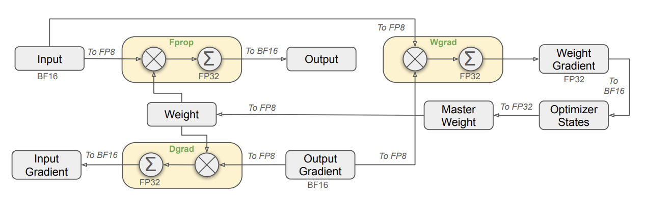
Note the precision of the optimizer state and master weight updates:

The weight gradient $g_t$ is output in FP32.
The optimizer states $m_{t-1}$ and $v_{t-1}$ are loaded from memory (as BF16) and cast up to FP32.
Optimizer state update in FP32
- $m_t = \beta_1 m_{t-1} + (1 - \beta_1) g_t$
- $v_t = \beta_2 v_{t-1} + (1 - \beta_2) g_t^2$
Bias correction in FP32
- $\hat{m}_t = m_t / (1 - \beta_1^t)$
- $\hat{v}_t = v_t / (1 - \beta_2^t)$
Update master weights in FP32
- $\theta_t = \theta_{t-1} - \eta \cdot (\frac{\hat{m}_t}{\sqrt{\hat{v}_t} + \epsilon} + \lambda \theta_{t-1})$
$m_t$ and $v_t$ are cast down to BF16 and written back to memory.

Improved quantization

With the mixed precision as a backdrop, DSV3 implements several ways to reduce quantization errors, mainly attributed to the lackluster dynamic range of FP8 leading to underflow/overflow. Each component in the framework behaves differently and hence we should adopt a personalized strategy for each component which is quantized: activations $X$ , weights $W$ , output gradient $dY$ . DSV3 introduces fine-grained quantization, beyond tensor scaling into block scaling. For activations ( $X$ and $dY$ ), the block size is 1x128 (i.e per token per 128 channels), for weights the block size is 128x128 (i.e per 128 input channels per 128 output channels). Something we haven't discussed previously when lifting block scaling is that new blackwell chips have a hardware supported datatype MXFP8 that uses a fixed 1x32 block size, this is directly mentioned in the DSV3 report "Notably, our fine-grained quantization strategy is highly consistent with the idea of microscaling formats (Rouhani et al., 2023b), while the Tensor Cores of NVIDIA next-generation GPUs (Blackwell series) have announced the support for microscaling formats with smaller quantization granularity (NVIDIA, 2024a)"

Typically, Fprop is performed using E4M3, and Dgrad and Wgrad in E5M2 for the increased dynamic range to avoid gradient underflow. DSV3 is able to adopt E4M3 for all its tensors, enabling higher precision. This feasibility is attributed to the fine-grained quant strategy of tile and block-wise scaling. Surprisingly, DSV3 employs online quantization, meaning the absolute value for each 1x128 activation tile or 128x128 weight block is computed online, based on each current tensor to derive the scaling factor used to quantize. This should severely reduce the observed gains from FP8.

Low precision storage and comms

Optimizer states are stored in BF16, master weights and gradients in FP32. As noted activations cached for the backward pass can be stored in FP8.

Increasing Accumulation Precision

Low-precision GEMM operations often suffer from underflow issues, and their accuracy largely depends on high-precision accumulation, which is commonly performed in FP32 precision. While working on DSV3, the team noticed that the FP8 GEMM on NVIDIA 800 GPUs was limited to retaining around 14 bits, significantly lower than FP32 accumulation precision. To address this, DSV3 adopts a particular promotion strategy within its CUDA cores for higher precision.

Sidebar: GPU Architecture

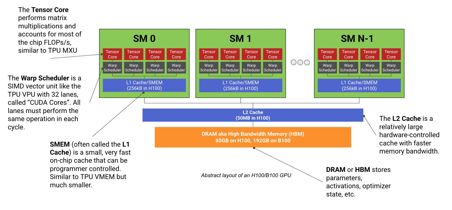
A GPU consists of a bunch of compute units, Streaming Multiprocessors (SM), attached to a fast stick of memory called HBM. A modern GPU such as a H100 as 132 SMs. Each SM contains dedicated matrix multiplication cores called Tensor Cores, vector arithmetic units (that is to say typical Arithmetic Logic Unit ALUs that do arithmetic and logic operations) called CUDA cores and chip cache (SMEM).

A SM consists of 4 identical SM subpartitions, each containing a Tensor Core, registers, and CUDA Cores. The CUDA Cores are a bunch of ALUs that perform scalar operations in a SIMT execution model. Each SM consists of 32 fp32 cores (and a smaller number of int32 and fp64 cores) that all axecute the same instruction in each cycle. However, CUDA cores use a SIMT (Single Instruction Multiple Threads) programming model as opposed to a normal SIMD model. The difference is that while all cores within a subpartition must execute the same operation in each cycle, each core (or "thread" in the CUDA programming model) has its own instruction pointer and can be programmed independently. The effect of this is that when two threads in the same warp (a warp is a group of 32 threads/cores that are bound together and function as a 32-wide SIMT unit) are instructed to perform different operations, you effectively do both operations, masking out the cores that don't need to perform the divergent operation.

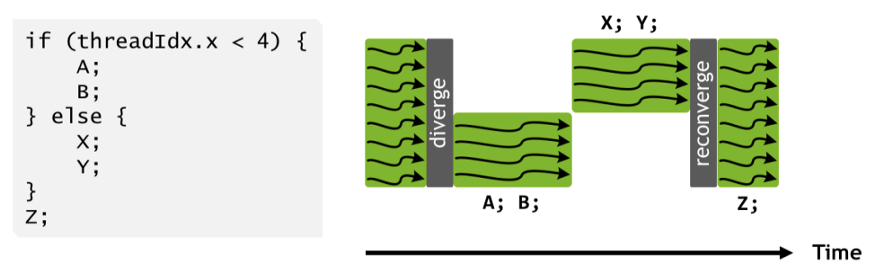
This enables flexible programming at the thread level, but at the cost of silently degrading performance if warps diverge too often.

Tensor Cores are the dedicated matrix multiplication unit, each SM subpartition has one. The Tensor Cores can perform lower precision matmuls at higher throughput.

DSV3's fine-grained quantization strategy introduces a per-group scaling factor along the inner (contracting) dimension of GEMM operations. This functionality was not directly supported in standard FP8 GEMM at the time. This required them to write a custom FP8-GEMM-with-rescaling kernel. This kernel efficiently solves both the per-group scaling and low-bit accumulation problem, which we'll detail next, with an overview figure shown first.

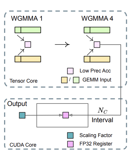
The GEMM runs a stream of WGMMA instructions on the Tensor Cores that perform Matrix-Multiply Accumulate in the restricted precision (14 bit) TC accumulator. After ~4 WGMMA issues (this maps to 128 elements of the K-reduction for the tile), we copy the TC partial sums into a separate register-backed accumulator tensor in FP32. Here we apply the appropriate scaling factors. Accumulation here is performed by CUDA Cores and thus takes place in ordinary FP32 precision. This gives is a clean way to apply our groupwise scaling factors (remember our scaling factors are 1x128 and 128x128) while simultaneously enabling high-precision accumulation. The GEMM can be expressed as

C=\sum_{g}\underbrace{\left(s_A^{(g)} s_B^{(g)}\right)}_{\text{dequant}}\cdot\underbrace{\sum_{k\in g} q_A[k],q_B[k]}_{\text{TC partial in low precision}}

The inner sum (per group $g$ ) is accumulated on Tensor Cores with limited precision; before errors grow too large, you promote and apply $s_A^{(g)} s_B^{(g)}$ in FP32 on CUDA cores and fold it into a high-precision FP32 accumulator.

summary

DSV3's leverages FP8 primarily for compute in its GEMMs, and less so to save memory. A considerable amount of compute is performed in FP8, most activations are cached in FP8, but in terms of model state most things use higher precision

Setup	Param	Grad	$m$	$v$	Bytes per parameter
DSV3	FP32 (4)	FP32 (4)	FP16 (2)	FP16 (2)	= 12 B

cuBLAS 12.9

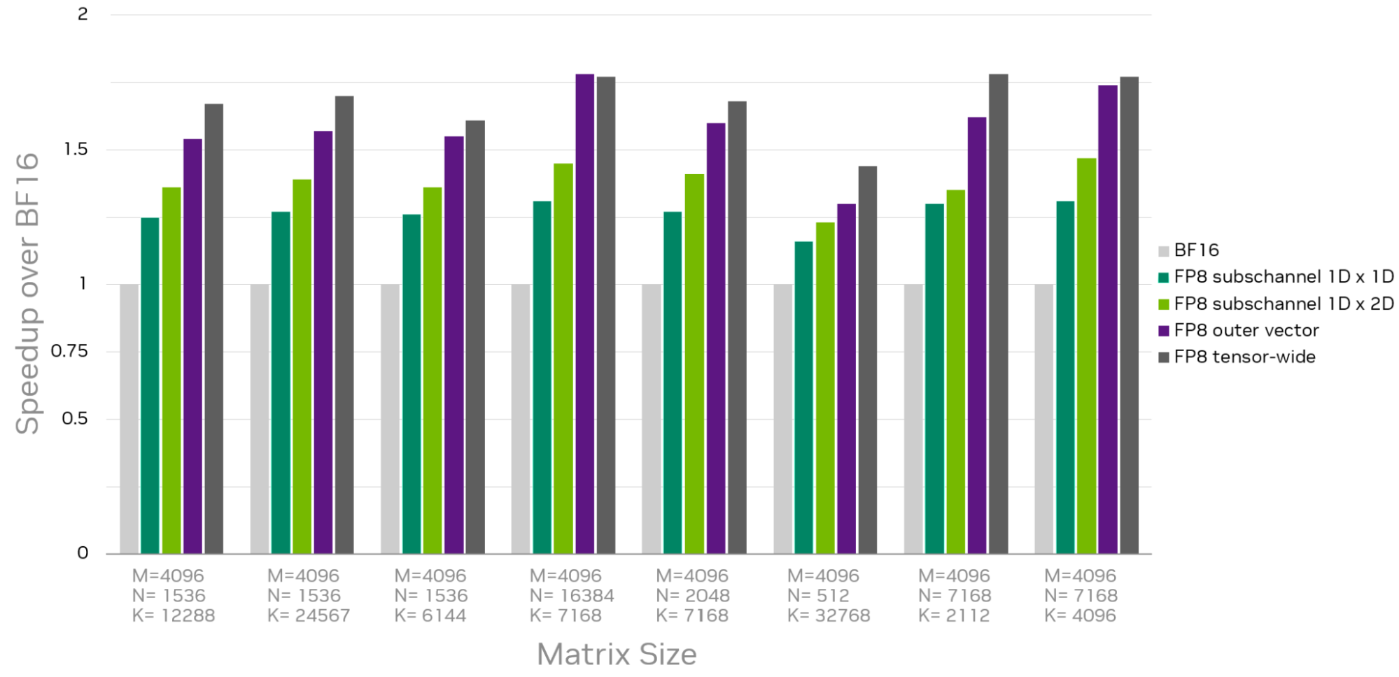
introduced new flexibility beyond the existing tensor-wise scaling for Hopper and Ada GPUs. Previous versions of cuBLAS only had tensor-wide scaling i.e. a single scaling factor, now you can apply channel-wide scaling factors enabling a single scaling factor to a individual matrix rows or columns. This can be further extended into block scaling, as used in DSV3. This allows you to apply a single scaling factor to each 128-element 1D block within the K dimension, or a 128x128 2D block. 1D blocks is higher accuracy and 2D blocks better performance.

Ling 2.0

Ling 2.0 adopts fine-grained quantization following DSV3. Beyond DSV3, the team aims to reduce memory footprint by quantizing certain model states into FP8, moving beyond what we saw in DSV3. The team is able to quantize both adam moments into FP8.

Kimi K2 Thinking

Aside from low precision training to both improve compute speed and memory pressure, there are two interesting paradigms that we have not covered. Post-training quantization, where weights of the trained model are quantized to a specific precision primarily to reduce memory pressure, and training-aware quantization which allows the model to pre-adapt to the precision loss caused by quantizing certain weights/activations to alower bit count during the training phase. These things are directly related to the inference side of things. For inference there are two different trade-off directions depending on your optimization objective:

High throughput (cost-oriented). The idea here is to maximize the throughput of your inference cluster, you do this by effectively utilizing your GPU compute resources, you want to be compute bound. This is achieved by massive parallelization such that you saturate your tensor cores. You achieve this through large batch size to make the GEMM compute bound.
Low lateny (user-experience orientated). The primary goal is to minimize the latency of a single inference request. This is a user facing approach. The objective is to reduce the output latency (TPOT) on the user side. This typically involves using relatively low concurrency and a small number of single-instance nodes.

K2 being a MoE with high sparsity (1/48) means they are highly memory bound during inference. The size of the model weights in memory determine the number of GPUs required, where fewer means lower multi-GPU comm latency. It just so happens that K2 at FP8 is just too big to be covered by NVLink connects, which significantly hampers intergpu comm speed. For such a reason the team really wanted to move to lower weight quantization, during the decodign stage the inference latency of W4A16 quantization is significantly better than W8A8.

For K2 the authors found that 4-bit PTQ was able to achieve near lossless performance across many benchmarks. However while working on K2-Thinking they observed significant statistical differences between FP8 model and INT4 PTQ, this was deemed to be linked to model length increasing. Additionally, PTQ is reliant on a calibration set. They tested some cases that appear in the training set but not in the PTQ calibration set and found that FP8 model was able to memorize these training data very well while the quantized model failed. The team guesses that when the moe is very sparse, even though the calibration set is large, some experts will still only be routed to a small number of tokens, leading to significant "distortion" in the quantization results of these experts. Ultimately they think that the way to achieve low bit inference for K2-thinking is through QAT.

QAT Solution

The used INT4 QAT isn't some "godlike technology", the team found that a relatively basic QAT solution easily achieves near lossless performance relative to baselines. The approach is weigh-only QAT, using a common fake-quantization + STE (direct-through estimator) approach. Original bf16 weights are preserved, obtain the weights after simulating the accuracy loss through quant-dequant, perform matmul, then directly update the bf16 weights during backprop.

INT4 is especially useful for RL, to address the issue of long tail problem in the rollout stage. With a INT4 model, the rollouts are faster and the long tail is less of a problem. Of course INT4 QAT requires quant-dequant during training which slightly increases training time but this is a small increase than the efficiency problem of rollout. Additionally, studies are now showing that quantized RL, introducing quantization noise during rollout may help creating more robust policies. Additionally they observe that at INT4 precision they see far less training-inference mismatch, likely due to the lower representation range of INT4 leading to less problems with accumulation order in diff kernels.

THe goal of QAT is to adapt the model to quantization numerics during training as to mitigate the inevitable quantization degradation when the model is actually quantized eventually, i.e for inference serving. This is achieved by simulating quantization numerics during training while keeping weights and/or activations in the original data type, effectively "fake quantizing" the values instead of actually casting them to lower bit-widths. This looks something like:

# PTQ: x_q is quantized and cast to int8  
# scale and zero point (zp) refer to parameters used to quantize x_float  
# qmin and qmax refer to the range of quantized values  
x_q = (x_float / scale + zp).round().clamp(qmin, qmax).cast(int8)  
  
# QAT: x_fq is still in float  
# Fake quantize simulates the numerics of quantize + dequantize  
x_fq = (x_float / scale + zp).round().clamp(qmin, qmax)  
x_fq = (x_fq - zp) * scale

From what the Kimi team themselves say, the process consists of during training you insert a fake quantize operations into the linear layers meaning that you quant-dequant weights prior to usage to simulate a quantization error, then perform the matmul as normal on the fake quantized weights. Since quantization involves non-differentiable operations like rounding, the QAT backward pass uses straight-through estimators, a mechanism to estimate the gradients flowing through non-smooth functions to ensure the gradients passes to the original weights are still meaningful. The output is calculated using fake quant weights but the gradients are calculate w.r.t the original weights i think. This way we gradients computed with the knowledge that the weights will be quantizied. During inference, model weights are stored in low-precision and dequantized prior to GEMM, which replicates the scenario seen during training.

PTQ

There are generally two kind of families of PTQ that you will find:

Weight-only (WoQ): Weights are stored in low bidwidth (INT4/INT8/FP8), activations stay in BF16/FP16. At runtime the kernel will dequant the packed weights to a higher precision compute type and run a standard GEMM, essentially F.linear(input, weight.to(input.dtype)), this mainly saves memory/bandwidth.
Weights + Activations (W8A8) Both sides are quantized and the matmul itself runs on low-precision tensor cores with higher-precision accumulation. This requires hardware support but is generally available on modern GPUs. This is the same methods that we see during training, where FP8 GEMMs are used.

There are a bunch of elaborate quantization schemes that fall inside these two family groups. Fror example bitsandbytes builds on the LLM.int8() paper which uses vector-wise quantization to quant Linear layers to 8-bits while using a separete "outlier" channel which are routed to a 16-bit matmul. There are also quantization schemes that are Weight-only but that use mixed precision kernels, Marlin is a very popular kernel library that implements extremely optimized INT4xFP16 matmul kernels for W4A16. This means weight-only schemes don't have to upcast and can use faster low-precision kernels. Activation quantization is either performed from a calibration set (static quantization) or dynamic (computed at run-time). Static quant is faster and enables fully integer kernels and dynamic is more robust but slower. There are also dynamic GGUF quants used by unsloth which use a calibration set to determine which weights in the model are more important and then assign more bits to these weights.