DeepSeek Sparse Attention

DeepSeek Sparse Attention (DSA) augments a standard transformer with a lightweight, parallel "lightning indexer." This indexer rapidly scores the entire token history and selects a small, top-$k$ set of the most relevant past tokens for each new query. The main, "core" attention mechanism—in DeepSeek's case, MLA—then operates only on this sparsely selected set. This approach dramatically cuts down on the compute required for long-context processing.

In DeepSeek's V3.2-Exp model, DSA is instantiated under MLA in a MQA configuration. This means each compressed, latent key-value entry is shared across all query heads. That being said, DSA's lightning indexer is compatible with any core attention variant.

Why DSA?

MLA (which we'll recap shortly) was by all means a pivotal optimization. It introduced a compressed KV cache, decoupling training and inference attention: models could leverage full MHA during training but run efficient MQA at inference. This design yields massive KV-cache savings while preserving high model quality. The problem, however, wasn't fully solved. The computation under MLA remains effectively equivalent to standard attention; the score calculation is still quadratic, $O(L^2)$ in sequence length.

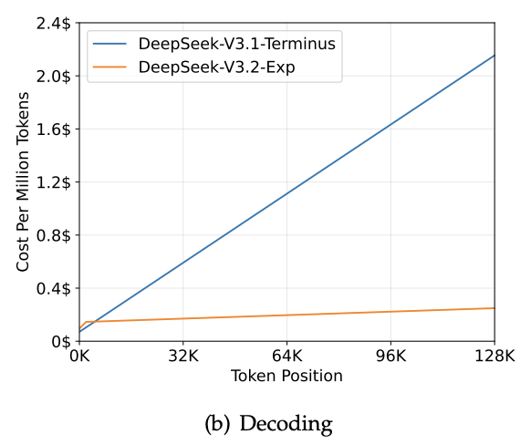
As context lengths grow—especially in complex, agentic settings—that $O(L^2)$ FLOPs cost quickly becomes the dominant bottleneck. 2025 has seen a wave of linear and sparse attention variants (we previously explored NSA at DeepSeek, but stable training has seemingly proved elusive for DS). DSA represents a more pragmatic and stable intermediate. It bridges the gap by using an extremely cheap indexer (few heads, small head dimension, FP8 precision) to select just $k$ surviving tokens. The expensive main attention mechanism then operates only on these $k$ survivors, bringing the core attention complexity down to $O(L \cdot k)$, where $k \ll L$.

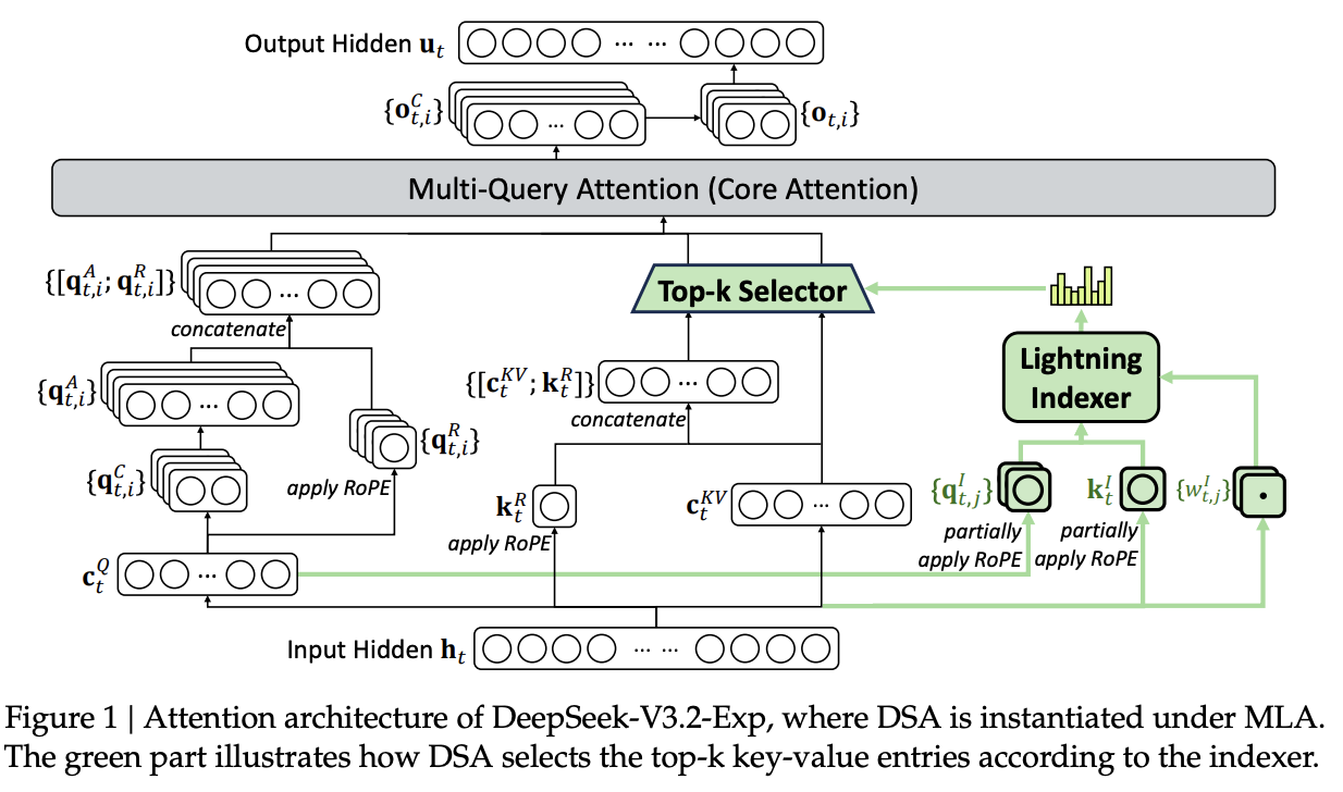
We'll anchor the rest of this post on the "DSA under MLA" architecture. The diagram below illustrates the two key paths: the new Lightning Indexer (the green path), which scans the history to produce index scores and a Top-$k$ selector, and the original Core Attention (the gray path), which now consumes only the $k$ selected latent KV entries. You can view this as a fast, compact search stage (the indexer) that gates a powerful but expensive attention stage (MLA); the indexer learns a compact metric space for similarity search, analogous to a learned k-NN.

To make sense of the integration, we first need to understand the baseline. We'll recap just enough of MLA to make the DSA modifications obvious, then walk through the indexer's design, connecting the math to the modeling code.

MLA

Let's first establish the MLA baseline. We enter the attention block with hidden states $x \in \mathbb{R}^{B \times S \times d_{\text{model}}}$. MLA's core idea is to factorize queries and keys into two complementary channels: a latent channel (which carries the content, or "what") and a RoPE channel (which carries the position, or "where"). Values live entirely within the latent channel.

The KV Path

First, we produce the key-value pre-activations via the "A" projection, $W^{KV}_{A}$. This tensor is immediately split into two parts: the latent KV ($c^{KV}$) and the RoPE key ($k^R$).

$$\tilde{k}^{A} = x W^{KV}_{A} \in \mathbb{R}^{B \times S \times (d_C + d_{\mathrm{RoPE}})}$$ $$\tilde{k}^{A} \Rightarrow c^{KV} \in \mathbb{R}^{B \times S \times d_C} \oplus k^{R} \in \mathbb{R}^{B \times S \times d_{\mathrm{RoPE}}}$$

Here, $d_C=\texttt{kv\_lora\_rank}$ is the dimension of the compressed latent KV, and $d_{\mathrm{RoPE}}=\texttt{qk\_rope\_head\_dim}$ is the head dimension of the decoupled RoPE key. The latent path is normalized, while the RoPE path gets its positional information.

$$c^{KV} \leftarrow \mathrm{RMSNorm}(c^{KV}) \qquad k^{R} \leftarrow \mathrm{RoPE}(k^{R})$$

# x: (B, S, d_model)
kvA = wkv_a(x)               # (B, S, d_C + d_RoPE)
cKV, kR = torch.split(kvA, [d_C, d_RoPE], dim=-1)  # (B,S,d_C), (B,S,d_RoPE)

# Apply norm and RoPE
cKV = kv_norm(cKV)
kR = apply_rotary_emb(kR, freqs_cis)   # (B,S,d_RoPE)

These two tensors are our entire key-value cache. For each token, we store just the compact content latent $c^{KV}$ and the decoupled positional key $k^{R}$.

kv_cache[:, start_pos:end_pos, :] = cKV  # (B, S, d_C)
pe_cache[:, start_pos:end_pos, :] = kR   # (B, S, d_RoPE)

The Query Path

On the query side, we do something similar. We first apply a low-rank "A" projection ($W^{Q}_{A}$) and normalize to get a compressed latent query, $c^Q$. (This $c^Q$ will be reused later by the lightning indexer, a key efficiency).

$$c^Q = \mathrm{RMSNorm}(x W^{Q}_{A}) \in \mathbb{R}^{B \times S \times d_Q}$$

# x: (B, S, d_model)
cQ  = q_norm(wq_a(x))        # (B, S, d_Q)

Here, $d_Q=\texttt{q\_lora\_rank}$ is the compressed query rank. To form the final per-head queries, we apply a second "B" projection ($W^{Q}_{B}$) from this latent $c^Q$, which expands it into $H$ heads. We then split each head into its no-RoPE ($q^A$) and RoPE ($q^R$) subspaces.

$$\begin{aligned} q &= c^Q W^{Q}_{B} \ &\Rightarrow \big(q^{A} \in \mathbb{R}^{B \times S \times H \times d_{\text{NoPE}}}, \ q^{R} \in \mathbb{R}^{B \times S \times H \times d_{\text{RoPE}}}\big), \end{aligned}$$ $$q^{R} \leftarrow \mathrm{RoPE}(q^{R})$$

# project to heads, then split
q_full = wq_b(cQ).view(B, S, H, d_NoPE + d_RoPE)
qA, qR = torch.split(q_full, [d_NoPE, d_RoPE], dim=-1)  # (B,S,H,d_NoPE), (B,S,H,d_RoPE)

# Apply RoPE only to the qR slice
qR = apply_rotary_emb(qR, freqs_cis)

Here, $d_{\text{NoPE}}=\texttt{qk\_nope\_head\_dim}$ and $d_{\text{RoPE}}=\texttt{qk\_rope\_head\_dim}$ sum to the full query-key head dimension $\texttt{qk\_head\_dim}$.

MLA "Trick"

Now we have our queries $\langle q^{A}, q^{R} \rangle$ and our cached keys $\langle c^{KV}, k^{R} \rangle$. A critical component of MLA is that we never materialize the full per-head keys for the entire history. Instead, we use an algebraic trick to score directly against the compact caches.

Consider the no-RoPE score contribution. If we did materialize the key for head $h$ at time $t$, we would take the latent $c^{KV}_t \in \mathbb{R}^{d_C}$ and apply the key-block of the "B" up-projection, let's call it $W_K \in \mathbb{R}^{d_{\text{NoPE}} \times d_C}$.

$$k^{\text{NoPE}}_{t} = W_K c^{KV}_t \in \mathbb{R}^{d_{\text{NoPE}}}.$$

The score would be the dot product with the query $q^A$:

$$\langle q^{A}, k^{\text{NoPE}}_{t} \rangle = q^{A\top} (W_K c^{KV}_t) = (W_K^\top q^{A})^\top c^{KV}_t.$$

This identity is the trick! Instead of projecting all $t$ past keys up ($W_K c^{KV}_t$), we project the single query $q^A$ down ($W_K^\top q^{A}$) and compute the dot product in the compact latent space $d_C$. We transform the query once so it can score directly against the $c^{KV}$ cache.

In code, this query transformation $\tilde{q} = W_K^\top q^{A}$ (named q_lat) looks a bit odd, but it's just a reshape and an einsum:

# wkv_b_weight is (H * (d_NoPE + d_V), d_C)
# We view it as (H, d_NoPE + d_V, d_C)
wkv_b = wkv_b_weight.view(H, d_NoPE + d_V, d_C)

# qA: (B, 1, H, d_NoPE)
# Take the first d_NoPE rows (the key block) for each head
q_lat = torch.einsum("bshd,hdc->bshc", qA, wkv_b[:, :d_NoPE])  # (B, 1, H, d_C)

The final scores are the sum of two dot products, both operating on the raw caches:

1. Latent Score: The transformed query q_lat dotted with the $c^{KV}$ cache.
2. RoPE Score: The RoPE query $q^R$ dotted with the $k^R$ cache.

# q_lat: (B, 1, H, d_C),  kv_cache: (B, t, d_C)
# qR:    (B, 1, H, d_RoPE), pe_cache: (B, t, d_RoPE)
scores = (
    torch.einsum("bshc,btc->bsht", q_lat, kv_cache[:, :t_end]) +  # latent: \tilde{q}^T c^{KV}_t
    torch.einsum("bshr,btr->bsht", qR,    pe_cache[:, :t_end])    # RoPE:  q^R · k^R_t
) * softmax_scale

Following the softmax, we aggregate the values in latent space using the same $c^{KV}$ cache. This keeps the heaviest computation (the weighted sum) in the compact $d_C$ dimension:

attn  = scores.softmax(dim=-1)                                   # (B, 1, H, t)
x_lat = torch.einsum("bsht,btc->bshc", attn, kv_cache[:, :t_end])  # (B, 1, H, d_C)

Finally, we expand this latent representation $x_{\text{lat}}$ to the full value head dimension $d_V$ using the value block of the $W^{KV}_B$ projection (the last $d_V$ rows) and project back to model space.

# Use the value rows (last d_V) per head to up-project
x_head = torch.einsum("bshc,hdc->bshd", x_lat, wkv_b[:, -d_V:])  # (B, 1, H, d_V)
x_out  = wo(x_head.flatten(2))                                   # (B, 1, d_model)

This latent trick is identical to standard attention but avoids ever constructing full per-head keys, saving memory and compute during the decode loop.

DeepSeek Sparse Attention (DSA)

MLA gave us compact per-token caches ($c^{KV}$ and $k^R$) and a decode path that avoids materializing full keys. What it didn't change is how many past tokens we touch: all $t$ of them, making the scoring $O(t)$.

The Lightning Indexer adds a fast, low-dimensional search stage before this scoring. It scans the entire history in a tiny, FP8-quantized space and proposes a top-$k$ candidate set. The expensive MLA scoring logic we just reviewed is then only run on those $k$ tokens.

Building the Indexer Space

The indexer builds its own compact space with $H_I = \texttt{index\_n\_heads}$ (e.g., 64) small heads of width $d_I = \texttt{index\_head\_dim}$ (e.g., 128). This space is separate from the main attention.

Indexer Query: The indexer query path starts from the same compressed query activation $c^Q \in \mathbb{R}^{B \times S \times d_Q}$ that MLA used. This is a key efficiency. We project it to the indexer's head space, split into NoPE and RoPE slices, and apply RoPE.

$$q^{\text{idx}} = c^Q W^{Q,\text{idx}}_{B} \in \mathbb{R}^{B \times S \times H_I \times \big(d_{I,\text{NoPE}} + d_{I,\text{RoPE}}\big)}$$ $$q^{\text{mix}} = \mathrm{concat}\big(q^{\text{idx}}_{\text{NoPE}},\ \mathrm{RoPE}(q^{\text{idx}}_{\text{RoPE}})\big) \in \mathbb{R}^{B \times S \times H_I \times d_I}$$

q_idx = wq_b_index(cQ).view(B, S, H_I, dI_NoPE + dI_RoPE)   # (B,S,H_I,·)
qI_nope, qI_rope = torch.split(q_idx, [dI_NoPE, dI_RoPE], dim=-1)
qI_rope = apply_rotary_emb(qI_rope, freqs_cis)
q_mix = torch.cat([qI_nope, qI_rope], dim=-1)                # (B,S,H_I,d_I)

Indexer Key: The same process is repeated for the keys, starting from the model hidden state $x$. However, the indexer key path is MQA-style (it's not split into heads), producing a single key vector per token.

$$k^{\text{mix}} \in \mathbb{R}^{B \times S \times d_I}$$

Hadamard Rotation: To decorrelate features and improve the numerical properties for low-precision math, both the queries and keys are rotated using a Walsh-Hadamard transform. Think of this as conditioning the vectors for a robust FP8 search.

$$q_{\text{rot}} = \mathrm{Hadamard}\big(q^{\text{mix}}\big), \qquad k_{\text{rot}} = \mathrm{Hadamard}\big(k^{\text{mix}}\big)$$

Scoring and Selection

The indexer runs entirely in FP8. Both the query and key activations are quantized, and the keys are cached in FP8 along with their per-block quantization scales.

$$(q_{\mathrm{fp8}}, s_q) = \mathrm{quant8}(q^{\text{rot}}), \qquad (k_{\mathrm{fp8}}, s_k) = \mathrm{quant8}(k^{\text{rot}})$$

q_fp8, q_scale = act_quant(q_rot)         # (B,S,H_I,d_I), (B,S,H_I,1 or blocks)
k_fp8, k_scale = act_quant(k_rot)         # (B,S,d_I),     (B,S,blocks)

# Update the FP8 indexer cache
k_cache[:, start:end]       = k_fp8
k_scale_cache[:, start:end] = k_scale

At decode time ($S=1$), a specialized fused kernel performs the search. This kernel runs an FP8 GEMM between the query $q_{\mathrm{fp8}}$ and the entire key cache $k_{\mathrm{fp8}, \le t}$. This is still an $O(t)$ operation, but the constants are tiny ($H_I$ and $d_I$ are small, and the math is FP8).

The kernel computes a nonnegative similarity (using a ReLU) for each head, then performs a weighted sum across the $H_I$ heads to produce a single scalar "index score" for each past token:

$$\text{logits}_{h,t} = q_{\mathrm{fp8},h} \cdot k_{\mathrm{fp8},t}$$ $$\text{logits}^{+}_{h,t} = \max\big(0,\ \text{logits}_{h,t}\big)$$ $$\text{score}_{t} = \sum_{h=1}^{H_I} w_h, \text{logits}^{+}_{h,t}$$ $$\text{index\_score}_{t} = \text{score}_{t} \cdot s_k(t)$$

Where $q_{\mathrm{fp8},h}$ is the FP8 query for indexer head $h$, $k_{\mathrm{fp8},t}$ is the FP8 key for token $t$, $\max(0,\cdot)$ is a ReLU that discards negative correlations, $w_h$ is a learned scalar gate (derived from the current $x$) that weights the importance of each indexer head and $s_k(t)$ is the per-block dequantization scale for key $t$, which restores the magnitude after the FP8 dot product.

# These weights are derived from x to combine heads cheaply inside the kernel
q_weights = head_weight_proj(x).view(B, S, H_I) * inv_sqrt(H_I)

# The fused fp8_index kernel does all the steps above:
# (B,S,H_I,d_I) @ (B,t,d_I) -> (B,S,t)
# It applies the ReLU, head weighting (q_weights), and k_scales internally.
index_score = fp8_index(
    q_fp8,                     # (B,S,H_I,d_I)
    q_weights,                 # (B,S,H_I)
    k_cache[:, :t_end],        # (B,t,d_I)    FP8
    k_scale_cache[:, :t_end],  # (B,t,blocks) per-block scales
)  # → (B,S,t)

Finally, we top-$k$ these scores to find the indices of the $k$ (e.g., 2048) most relevant tokens.

The complete DSA loop is as follows:

1. Build compact FP8 search vectors (Q and K) for the indexer.
2. Run a fast, fused FP8 search to score all $t$ past tokens.
3. Select the top-$k$ token indices.
4. Pass only these $k$ indices to the main MLA attention layer, which performs its expensive $O(k)$ scoring and aggregation.

By filtering the history, DSA lets MLA operate on a tiny fraction of the full context, achieving massive computational savings while maintaining high performance.