Ling 2.0 and MoE Scaling Laws

The Ling Team operates within inclusionAI, an organization housing open-source projects from Ant Group, the Chinese fintech company best known for Alipay. This team, essentially another of Alibaba's research groups dedicated to AGI. On their github we read: This organization contains the series of open-source projects from Ant Group with dedicated efforts to work towards Artificial General Intelligence (AGI). And they've really been making a ton of interesting moves in the dark.

Today, we'll first take a look at a scaling laws paper from the Ling Team, published mid summer, then we'll discuss the subsequent product of these scaling laws which is the Ling 2.0 model family.

MoE glossary

Total and Active Parameters. In MoE models, we distinguish between the total parameters of the model and the number of parameters active in the forward pass, due to the top-k gating mechanism of experts.

Routable and Sharable Experts. An MoE layer typically has a total number of routable experts $E$, from which the gating network selects a subset of $E_a$ (num activated experts) for each token. Additionally, many MoE architectures incorporate $E_s$ shared experts which are experts every token is routed through. These shared experts free the routable experts from having to encode overlapping features.

Activation Ratio and Sharing Ratio. There are two metrics that characterize the expert configuration. Activation ratio, $A$, is the ratio of activate experts to the total number of experts $A = (E_a + E_s) / (E + E_s)$, and sharing ratio is the ratio of shared experts to activated experts $S = E_s / (E_a + E_s)$. Together these metrics define the sparsity of our MoE layer.

Granularity of Experts. Prior to DeepSeek, it was common practice for the intermediate dimension of each expert to be equal to the FFN hidden dimension, which was typically around 2~4 x d_model. However, now adays we commonly see these two dimensions decoupled from each other, meaning we have a expert dimension and a FFN dimension. To analyze this design choice, the authors define expert granularity as $G = 2d_\text{model} / d_\text{expert}$. A higher value of G corresponds to having a larger number of smaller experts for a fixed total parameter count within the MoE layers.

Defining Model Scale via Computation. This work quantifies the computational cost through FLOPs. A model's scale, denoted $M$, represents the number of non-embedding FLOPs per token in a single forward pass. For MoE models this is especially important because $M$ only depends on the activated parameters of the architecture, i.e the selected experts. Total training compute is defined as $C = M \cdot D$.

Scaling laws for Hparams and Data allocation

The paper first establishes scaling laws for batch size and learning rate as a function of total compute $C$. The authors perform a hyperparameter search over a compute range of 3e17 to 3e20 FLOPs. These experiments use a fixed MoE configuration with $E=64$ routable experts, $E_a=4$ activated experts, and $E_s=1$ shared expert, resulting in an activation ratio $A=7.8\%$ and a granularity $G=2$. The fitting process yields the following formulas:

$$\begin{align} n^\text{opt} &= 1.1576 \cdot C^{-0.1529} \\ B^\text{opt} &= 0.0694 \cdot C^{0.3644} \end{align}$$

As mentioned, these laws are derived from a single configuration of the MoE layer, so we need to verify the generalization of these laws to other archs, specifically ones with alternative activation ratios. To test this, the derived laws are used to predict optimal hyperparameters at a compute budget of 3e20 FLOPs, after fitting them on data up to 1e20 FLOPs. Performing these experiments they find that the predicted optimal regions effectively capture the best-performing hyperparameters for activation ratos from 4.7% to 10.9% demonstrating that these laws can be applied to MoE models within this range. For reference a bunch of activation ratio for recent MoE models:

These laws are derived from a single MoE configuration, so their generalizability requires verification. The authors test this by using the laws to predict optimal hyperparameters at a compute budget of 3e20 FLOPs (after fitting on data up to 1e20 FLOPs). The predictions effectively capture the best-performing hyperparameters for activation ratios from 4.7% to 10.9%. This range covers many recent MoE models:

Model	Activation Ratio
Kimi K2	2.3%
Deepseek V3.1	3.5
Qwen 3	6.25%
GLM 4.5	5.59%
Ling 2.0	3.1%

I appreciate the validation, but testing at just a single compute point ($C=3\text{e}20$) feels insufficient to claim universal invariance across all activation ratios and budgets. To me, it seems slightly optimistic to claim universality of these laws, and invariance "across activation ratios and budgets".

What about model/data allocation? Classic scaling law papers for dense models guide how to allocate a fixed compute budget between model size and data volume. The problem is formally defined as:

$(M^{\text{opt}}, D^{\text{opt}}) = \arg\min_{M,D} \; \mathcal{L}(M,D; C, A, G, S) \quad \text{s.t.} \quad C = M \cdot D$

The derived scaling laws for MoE models are fairly similar to those for dense models. For MoEs, we have

$$\begin{align} M^\text{opt} &= 0.1915 \cdot C^{0.5095} \\ D^\text{opt} &= 5.2232 \cdot C^{0.4905} \end{align}$$

whereas for dense models

$$\begin{align} M^\text{opt} &= 0.0655 \cdot C^{0.5422} \\ D^\text{opt} &= 15.2582 \cdot C^{0.4578}. \end{align}$$

This suggests optimal MoE models are slightly smaller (lower $M^{\text{opt}}$) but are trained on more data than their dense counterparts. Both have exponents close to 0.5, indicating that additional compute should be split evenly between model and data scaling.

However, these allocation experiments were also derived from a single, fixed MoE architecture ($A=7.8\%$, $G=2$), and this time without validation across other architectures. The paper's premise is that MoE architecture (defined by $A$, $G$, etc.) determines a model's "effective capacity." It follows that the optimal model-data trade-off should also depend on this capacity. By using a single architecture to derive these laws, the subsequent experiments in might not be in the compute-optimal regime for configurations that differ significantly from the reference. While these experiments are expensive, this is a notable limitation.

Efficiency Leverage

is defined to quantify the computational efficiency gain of MoE compared to dense models. Using loss as our measure of performance, we can imagine that the required compute $C$, to achieve a certain loss as the most straightforward measurement of efficiency. Let $\mathcal{X}_{\text{Dense}}$ denote a standard dense architecture, and $\mathcal{X}_{\text{MoE}}$ represent a MoE architecutre. Models within $\mathcal{X}_{\text{MoE}}$ share the same activation ratio, granularity, shared experts and are scaled solely through increased hidden dimensions ($d_\text{model}$, $d_\text{ffn}$, $d_\text{expert}$) and number of layers. Determining the compute at which a certain loss is achieved under these two model architectures $\mathcal{L}(C_{\text{dense}}; \mathcal{X}_{\text{Dense}})$, $\mathcal{L}(C_{\text{moe}}; \mathcal{X}_{\text{MoE}})$; gives us a comparable metric by which we can determin efficiency. Formally, efficiency leverage is defined as:

$$EL(\mathcal{X}_{\text{MoE}} \mid \mathcal{X}_{\text{Dense}}; C_{\text{target}}) = \frac{C_{\text{dense}}}{C_{\text{moe}}}, \quad \text{s.t.} \quad \big| \mathcal{L}(C_{\text{moe}}; \mathcal{X}_{\text{MoE}}) - \mathcal{L}(C_{\text{dense}}; \mathcal{X}_{\text{Dense}}) \big| \leq \epsilon \quad (\epsilon \to 0)$$

An EL greater than 1 signifies that the MoE architecture is more computationally efficient than its dense counterpart. With this metric, the study investigates how activation ratio, expert granularity, and shared expert ratio affect EL, aiming to find the configuration $(A, G, S)$ that maximizes EL for a given compute budget. The experiments vary one dimension at a time from a baseline MoE architecture (2 of 64 experts activated, one shared expert).

From the results in the previous section we've already concluded the optimal batch size, learning rate, model and data allocation given a compute budget, which means that we can scan across different activation ratios, granularities and shared expert ratios, while holding other factors and the model scale M constant, and know the setup to train said model architecture at near its peak potential for a given budget, yielding reliable and cost effective conclusions. Since we've already derived scaling laws for dense models, it is easy to calculate the EL of each MoE configuration.

Activation Ratio

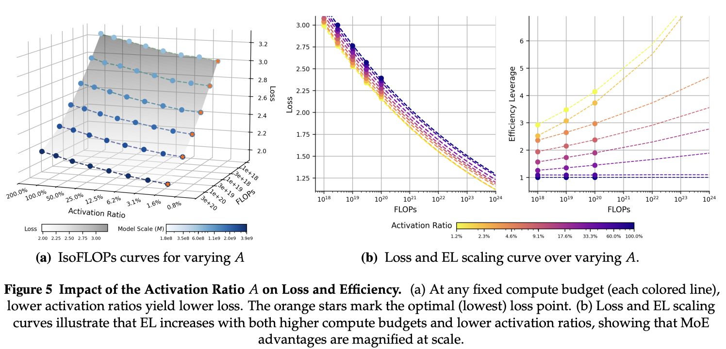
Experiments reveal that, at a fixed compute budget, loss monotonically decreases as the activation ratio decreases. The lowest tested ratio of 0.8% consistently yields the minimum loss. This implies a clear trade-off: greater MoE sparsity should be compensated for with larger hidden dimensions ($d_{\text{model}}$, $d_{\text{ffn}}$, $d_{\text{expert}}$) to maximize performance. When fitting loss scaling curves, the results show that EL consistently increases with lower activation ratios and grows with the total compute budget, demonstrating that the MoE advantage is amplified at larger scales.

These findings align with the Kimi K2 technical reports, which also found that under a fixed number of activated parameters (constant FLOPs), increasing the total number of experts (i.e., decreasing the activation ratio) consistently lowers loss up to a sparsity factor of at least 64 (1.56% activation ratio). However, Kimi K2 stops at a sparsity of 48 (2.1% activation ratio), citing infrastructure complexity as a practical constraint.

Granularity

Recalling that granularity is $G = 2d_{\text{model}} / d_{\text{expert}}$, experiments hold model size and activation ratio constant by increasing the number of experts while proportionally decreasing their size. This allows for testing granularities from 2 to 16. For reference, granularities of modern MoEs are typically lower:

Model	Granularity
Kimi K2	7
DeepSeek V3.1	7
Qwen 3 235B	5.33
Qwen 3 30B	5.33
GLM 4.5	6.67

The IsoFLOPs curves reveal a polynomial relationship between granularity and training loss. Loss first decreases as granularity increases, reaches a minimum, and then begins to increase. An optimal granularity of around 12 remains stable across a wide range of FLOPs budgets—much higher than what is common today. The authors note, however, that poor routing balance shifts this optimum toward coarser granularities (fewer, larger experts).

Shared Expert Ratio

Here, the total number of active experts ($E_a + E_s$) and the activation ratio are fixed, while routed experts are substituted for shared ones. The optimal shared expert ratio depends on the compute budget. Generally, a low, non-zero ratio minimizes loss. For lower compute budgets ($<10^{20}$ FLOPs), a slightly higher ratio ($S=16.7\%$) is beneficial, while for larger budgets ($>10^{20}$ FLOPs), a lower ratio ($S=8.3\%$) is more efficient. Since today's pre-training runs typically exceed $10^{20}$ FLOPs, the practical heuristic is to use a single shared expert.

Ling 2.0

It's always satisfying to see theory translate into practice. Following the publication of their scaling laws, the Ling team released the Ling 2.0 family, a series of MoE models built entirely on these findings.

The Ling 2.0 series includes several models. The first to be released was Ling-mini-2.0, a 16B total parameter MoE model with 1.4B active parameters. It was released as both a base model and a fine-tuned version called Ring-mini-2.0, which focuses on reasoning and appears to be trained with a mix of SFT, RLVR, and RLHF. More recently, the team released the larger Ling-flash-2.0, a 100B model with 6.1B active parameters.

As expected, the architectural choices for these models are grounded in the paper's scaling laws. For example, they use an activation ratio of 1/32 (~3%) and a granularity of 8. While the paper identified a theoretical optimum granularity of around 12, this choice likely reflects a practical trade-off. As their research noted, the benefits of finer granularity are highly dependent on robust expert routing; a slightly coarser granularity of 8 may offer a better balance between performance and training stability, mitigating the risks of routing imbalance.

Expert Routing

The original DeepSeekMoE architecture used softmax-based gating, where the gate value is given by

$$\text{Softmax}(W_g h_t)$$

where $W_g$ is a learnable matrix and $h_t$ is the input to the FFN representing the hidden state of a token.

This changed slightly in DeepSeek V3, with softmax gating being switched to sigmoid gating.

DeepSeekMoE

$$g_{i,t} = \begin{cases} s_{i,t}, & s_{i,t} \in \text{Topk}(\{s_{j,t} \mid 1 \leq j \leq mN\}, mK) \\ 0, & \text{otherwise} \end{cases}$$ $$s_{i,t} = \text{Softmax}_i \left( \mathbf{u}_t^T \mathbf{e}_i \right)$$

DeepSeek V3

$$g_{i,t} = \frac{g'_{i,t}}{\sum_{j=1}^{N_r} g'_{j,t}}$$ $$g'_{i,t} = \begin{cases} s_{i,t}, & s_{i,t} \in \text{Topk}(\{s_{j,t} \mid 1 \leq j \leq N_r\}, K_r) \\ 0, & \text{otherwise} \end{cases}$$ $$s_{i,t} = \text{Sigmoid} \left( \mathbf{u}_t^T \mathbf{e}_i \right)$$

Note that when using softmax, the resulting gates $\sum g_{i,t} < 1$. In DeepSeek V3 this was swapped to a sigmoid, not forcing the affinity scores to sum to 1, and instead performing normalization after the top-k affinity scores are selected to produce the final gating values. The same expert routing is used in V3.1.

Ling 2.0 uses the same V3 style of expert routing, with sigmoid to determine affinity scores and normalization applied after the top-k scores are retrieved.

Ling-flash-2.0

Was released just a few days ago, again building on the Ling 2.0 architecture, which in turn built on the findings of the scaling law papers.

I’ve removed some of the uninteresting parts of the config so we can talk about the architecture:

{
  "architectures": ["BailingMoeV2ForCausalLM"],
  "num_hidden_layers": 32,
  "hidden_size": 4096,
  "intermediate_size": 9216,
  "first_k_dense_replace": 1,
  "hidden_act": "silu",
  "model_type": "bailing_moe",
  "moe_intermediate_size": 1024,
  "norm_topk_prob": true,
  "num_experts_per_tok": 8,
  "num_attention_heads": 32,
  "num_experts": 256,
  "num_key_value_heads": 4,
  "tie_word_embeddings": false,
  "head_dim": 128,
  "num_shared_experts": 1,
  "vocab_size": 157184,
  "moe_router_enable_expert_bias": true,
  "routed_scaling_factor": 2.5,
  "n_group": 8,
  "topk_group": 4,
  "use_qk_norm": true,
  "score_function": "sigmoid",
  "moe_shared_expert_intermediate_size": 1024
}

The to note are:

• Standard SwiGLU FFN
• GQA, with 8 groups.
• First block = dense FFN
• Vocab = 157k
• Multi-token prediction training
• 256 experts
• only 32 attention heads