beyond chinchilla - embracing a world of inference

Gone are the days where language models are mere research prototypes, tucked away in academic corridors and accessed by a select few. Today, LLMs are products, optimized to cater to the vast and varied demands of the public. While the scaling laws laid down by Kaplan and Chinchilla have been instrumental in this evolution, they're starting to show their limits as the industry veers away from them. The crux of the issue lies in the fact that these scaling laws primarily focus on pre-training compute costs, overlooking the significant expenses incurred during inference in today's computational ecosystem. So, what's prompting this shift away from Chinchilla's path, and how do we adeptly navigate this evolving terrain? It's time to delve into these questions and uncover the nuances of efficiently scaling LLMs in a inference-dominated world.

A first step from Chinchilla-optimal

Training models according to the Chinchilla scaling laws may be optimal from a training perspective, but LLMs are rarely developed just for display; they are meant to be utilized, which incurs inference costs. Consequently, it has become popular to train smaller models for extended periods, contrary to what Chinchilla laws would suggest, because smaller models entail cheaper inference. Leveraging these scaling laws, we can understand the trade-off between model size and compute overhead, leading to an insight into the critical model size. This size is the minimum necessary to achieve a certain loss. Such calculations are crucial as they determine the computational overhead for practitioners aiming to train a smaller model to the same loss level as a larger alternative.

Model size - compute overhead tradeoff

The complete derivation of the formulas discussed can be found here. I'll focus on the results and their implications. As a refresher, the Chinchilla paper modeled the loss as:

$$L(N,D) = E + \frac{A}{N^\alpha} + \frac{B}{D^\beta}.$$

Through a series of experiments, the authors determined parameter constants $E$, $A$, $B$, $\alpha$ and $\beta$. The final loss, as a function of parameter count $N$, and dataset tokens $D$ can be visualized as:

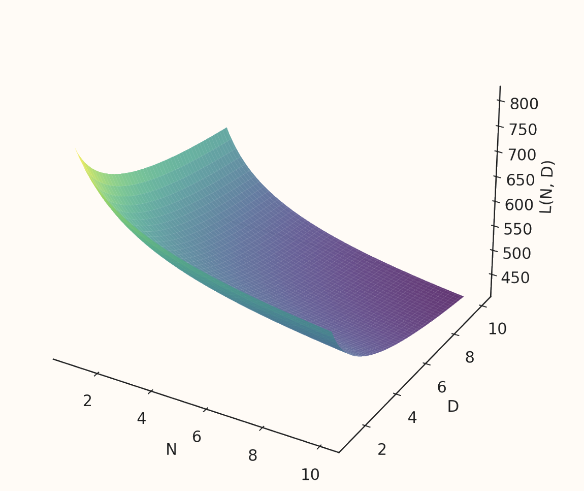
As familiar, increasing parameters and / or data leads to a decrease in the final loss. Notice however that the relationship is skewed towards data, meaning that a certain loss will be achieved quicker by scaling data more than model size. If you optimize this loss function you can calculate the optimal $N_{opt}$, $D_{opt}$, for a given compute (if any of this feels unfamiliar, see here). This is all well and good, but what if you want to train a sub-optimal model, smaller than chinchilla optimal for a given compute? Scaling the model by a parameter scale $k_N$ and a data scale $k_D$, the compute for this model:

$$C_{new} = 6(k_NN_{opt})(k_DD_{opt}),$$

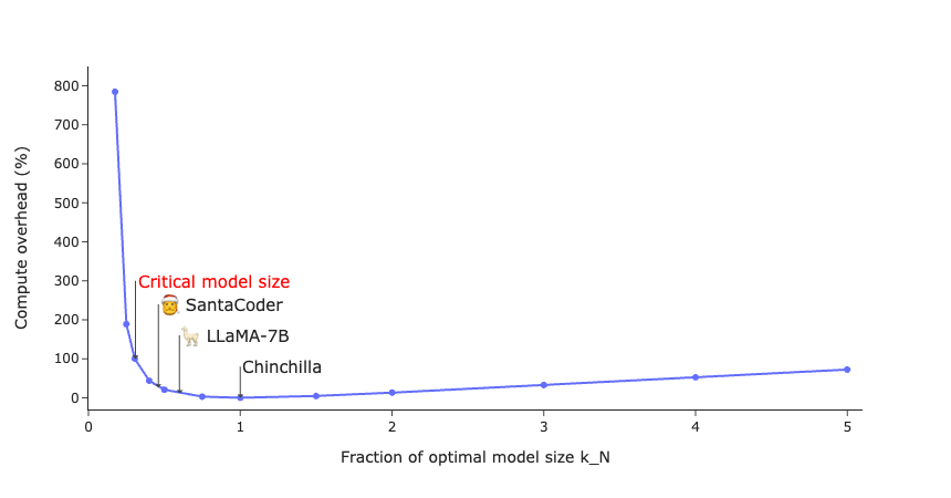
becomes proportional to the optimal. This means that if we want to train a smaller model $N < N_{opt}$, we need scale our training tokens inversely $D > D_{opt}$ to reach the same loss. Naturally, training for longer occurs additional overhead, calculated as

$$C_{overhead} = \frac{C_{new} - C}{C} * 100.$$

This relationship is visualized in the figure below, where chinchilla is represented as $k_N = 1$ with $C_{overhead} = 0$.

Critical model size

As depicted in the figure, there exists a substantial region below the As illustrated, there is a significant region below the optimal model size where the compute overhead is minimal. As we move towards smaller models, the compute overhead escalates exponentially. The critical model size is approximately 30% of Chinchilla's size, with a compute overhead of 100%. This doesn't imply that scaling down further is impossible; it just means that the returns diminish. It's important to remember that this 30% is relative to what the Chinchilla scaling laws suggest for a given compute. Where you position yourself on this curve depends on your inference demands.

Mixing in inference demands

The aforementioned conclusions are insightful, but what if we want our scaling laws to consider inference costs? The previous calculations give a rough estimate of the compute overhead required to train smaller models to a certain loss point. However, they don't factor in the eventual inference costs that a served LLM will incur. Fortunately, a new paper from two authors at MosiacML, "Beyond Chinchilla-Optimal: Accounting for Inference in Language Model Scaling Laws" offers assistance!

Their objective is to integrate inference costs into the model for pre-training loss, which we're already familiar with:

$$L(N,D_{\text{tr}}) = E + \frac{A}{N^\alpha} + \frac{B}{D_{\text{tr}}^\beta}.$$

---

It should be noted that the established constants $E$, $A$, $B$, $\alpha$ and $\beta$ depend on model architecture and dataset. However, the authors have chosen to use the same constants as they have been found consistent in subsequent research.

---

The authors use pre-training cross-entropy loss (formalized above) as a proxy for model quality and floating-point operations (FLOPs) as the unit of computational cost. Let $T_{FLOPs}(N,D)$ and $I_{FLOPs}(N,D)$ represent the number of FLOPs required for training and inference, respectively. $D_{inf}^{(i)}$ denotes the number of tokens per inference request. Formally, the aim is to minimize the sum of training and inference FLOPs (cost) for a given loss (quality), $\ell$:

$$N^*(\ell,D_{\text{inf}}), D_{\text{tr}}^*(\ell, D_{\text{inf}}) = \arg\min_{N, D_{\text{tr}} | L(N, D_{\text{tr}}) = \ell} \text{T}_{FLOPs} (N, D_{\text{tr}}) + \sum _i \text{I}_{FLOPs} (N, D_{\text{inf}}^{(i)}).$$

This might look scary, but don't worry let's break it down! The objective we are looking to minimize:

$$\text{T}_{FLOPs} (N, D_{\text{tr}}) + \sum _i \text{I}_{FLOPs} (N, D_{\text{inf}}^{(i)})$$

is the cost of pretraining, plus the cumulative cost of all inference requests. We are minimizing this under the condition:

$${N, D_{\text{tr}} | L(N, D_{\text{tr}}) = \ell}.$$

This condition signifies our aim to find the optimal number of model parameters $N$ and the amount of pretraining tokens $D$ that minimize the aforementioned objective, while ensuring the loss function $L(N,D_{\text{tr}})$ meets a certain quality, $\ell$. The optimization function takes a loss, $\ell$ and inference demand $D_{\text{inf}}$ as input.

Using the standard approximation of FLOPs for transformer models with $N$ parameters ($6N$ for training and $2N$ for inference), the objective simplifies to

$$N^*(\ell,D_{\text{inf}}), D_{\text{tr}}^*(\ell, D_{\text{inf}}) = \arg\min_{N, D_{\text{tr}} | L(N, D_{\text{tr}}) = \ell} 6ND_{\text{tr}} + 2ND_{\text{inf}}.$$

Note that, as opposed to the Chinchilla optimization problem where compute is fixed and the goal is to minimize pre-training loss, this problem fixes pre-training loss and finds $N$, $D$ that minimize compute costs. However, this reformulation relies on the assumption that practitioners can estimate their inference demand prior to training. The figure below shows how the inference-adjusted model's FLOP counts, parameters, and pre-training tokens compare to Chinchilla-optimal across various loss values and inference demands.

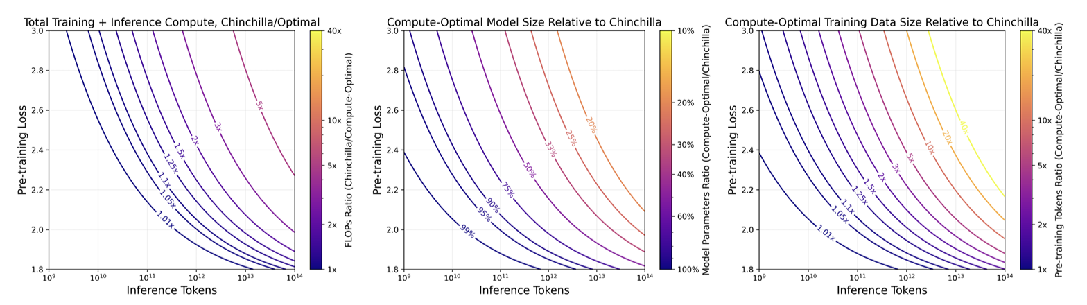
A practitioner that expects a 30B-Chinchilla quality model (~1.95 loss), with $10^{13}$ tokens in inference demand can reduce their total costs by 28% by training a 13.6 model on 2.84x the data. It's clear that the as inference demand approaches pre-training data size, the additional cost push the optimal parameter-to-token ratio towards smaller models trained for longer. This in itself isn't groundbreaking, but we know how away to approximate this relationship before training our models, something that is crucial when training runs can run up millions of dollars.