Mistral 7B

Original paper · Jiang et al 2023

Mistral 7B has quickly become the darling foundational model of the open source community, surpassing that of LLama 2 in a lot of regards. Mistral 7B has become the favorite OSS base model to use for further development, taking the spot that LLama 2 previously occupied. While it's important to not forget that this is still a 7B model, the capabilities of some of the models stemming from Mistral is amazing. New Mistral-derived models are being published almost daily. User u/WolframRavenwolf has published several in-depth evaluations of instruction-tuned open-source models; going beyond the standard benchmarks. I highly recommend you check them out, he's dedicated some serious time to provide this to the OSS community [1,2,2]. As Wolfram himself states, Mistral 7B just keeps getting better. People love it and are frequently pushing it to new heights, there's was even a 128k context version published just a few days ago!

Unpacking Mistral 7B's Appeal

Naturally, one starts to wonder what's special about Mistral 7B. Well, let's dive into some of the specific implementation details. Architecturally the model is quite similar to LLama, not a huge surprise considering that three of the co-authors of this paper (also founders of Mistral) authored the original Llama paper. But, what did they change this time around?

Decoding Sliding Window Attention (SWA)

The paper is overall quite thin and leaves out a lot of the details behind their implementation. This annoyed me because I couldn't quite grasp the fundamentals behind Sliding Window Attention. How does the context window expand theoretically without increasing computation? What is being attended to in each separate transformer layer? A lot of questions, little answers. As such, I'm going to do my best to demystify SWA.

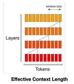
The elevator pitch of SWA sounds something like this: Vanilla attention requires time and memory that grow quadratically with the sequence length (linear memory thanks to FlashAttention). SWA employs a fixed-size window attention to $W$ preceding tokens. Multiple stacked layers of such windows attention results in a large receptive field where top layers have access to all input locations, similar to CNNs. If you are familiar with WaveNet, this should ring a bell. Unfortunately, my penny still hadn't dropped. Instead, let's walk through a practical example of SWA!

Consider the input sequence "A boy went to the shop" with a window size of 2. We'll assign scalar embeddings to each token and use an average operation across the window to simulate attention. While this is an abstraction from the traditional query, key, and value vectors, it allows us to focus on the core idea: computing output values from the tokens within the window. Remember, the fundamentals are still the same, we're still computing the resulting value from the tokens inside the window. Lastly, by layers we mean attention layers, we only care about the attention part of the architecture right now. My example is meant to illustrate Figure 1 of the paper, shown below.

Input sequence = "A boy went to the shop"
Window size = 2

Assigning simple scalar embeddings:

A: [0.1]
boy: [0.2]
went: [0.3]
to: [0.4]
the: [0.5]
shop: [0.6]

Computing the attended values for Layer 1:

"A" has no previous token, so it remains [0.1].
"boy" averages its value with "A": (0.2 + 0.1) / 2 = [0.15]
"went" averages with "boy": (0.3 + 0.2) / 2 = [0.25]
"to" averages with "went": (0.3 + 0.4) / 2 = [0.35]
"the" averages with "to": (0.4 + 0.5) / 2 = [0.45]
"shop" averages with "the": (0.5 + 0.6) / 2 = [0.55]

Let's illustrate this

Layer / Token	A	boy	went	to	the	shop
L1	0.1	0.15	0.25	0.35	0.45	0.55

Here's the representation of the context that each token attends to

Layer/Token	A	boy	went	to	the	shop
L1	[A]	[A, boy]	[boy, went]	[went, to]	[to, the]	[the, shop]

Remember that in a normal Transformer decoder, the representation would look like this

Layer/Token	A	boy	went	to	the	shop
L1	[A]	[A, boy]	[A, boy, went]	[A, boy, went, to]	[A, boy, went, to, the]	[A, boy, went, to, the, shop]

In the earlier layers, the attention is heavily restricted, but let's check out what happens as the sequence moves on to Layer 2.

Computing the attended values for Layer 2:

"A" has no previous token, so it remains [0.1].
"boy" averages its value with "A": (0.15 + 0.1) / 2 = [0.125]
"went" averages with "boy": (0.25 + 0.15) / 2 = [0.2]
... and so on.

The first two retain their context, but things get interesting when we look at the context for the succeeding values.

Layer/Token	A	boy	went	to	the	shop
L1	[A]	[A, boy]	[boy, went]	[went, to]	[to, the]	[the, shop]
L2	[A]	[A, boy]	[A, boy, went]	[boy, went, to]	[went, to, the]	[to, the, shop]

Notice how "went" representation is influenced by [A, boy, went] indirectly through "boy" representation [A, boy]! The compiled values:

Layer/Token	A	boy	went	to	the	shop
L1	0.1	0.15	0.25	0.35	0.45	0.55
L2	0.1	0.125	0.20	0.30	0.40	0.50

Sliding Window Attention exploits the stacked layers of transformers to attend to information beyond the window size. The context representation and values through 4 layers are shown below.

Layer/Token	A	boy	went	to	the	shop
L1	[A]	[A, boy]	[boy, went]	[went, to]	[to, the]	[the, shop]
L2	[A]	[A, boy]	[A, boy, went]	[boy, went, to]	[went, to, the]	[to, the, shop]
L3	[A]	[A, boy]	[A, boy, went]	[A, boy, went, to]	[boy, went, to, the]	[went, to, the, shop]
L4	[A]	[A, boy]	[A, boy, went]	[A, boy, went, to]	[A, boy, went, to, the]	[boy, went, to, the, shop]

Layer/Token	A	boy	went	to	the	shop
L1	0.1	0.15	0.25	0.35	0.45	0.55
L2	0.1	0.125	0.20	0.30	0.40	0.50
L3	0.1	0.1125	0.1625	0.25	0.35	0.45
L4	0.1	0.10625	0.1375	0.20625	0.30	0.40

The values represent a gradual blending of context: starting with individual token values, each subsequent layer averages these within a window, spreading the influence of early tokens (like "A") through the sequence. At each attention layer, information can move forward by $w$ tokens. Hence, after $k$ attention layers, information can move forward by up to $k \times W$ tokens. Our example simplifies attention to equal weighting across tokens, abstracting away more nuanced weighting variations, but effectively demonstrates local context aggregation in the Sliding Window Attention mechanism.

Grouped Query Attention

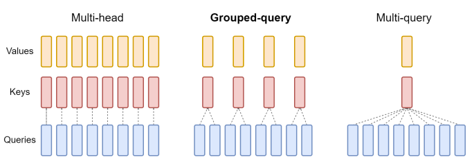
One of the bottlenecks in decoder performance is the memory bandwidth overhead incurred from repeatedly loading decoder weights and attention keys/values during each step of decoding. Multi-query Attention (MQA), which only uses a single key-value head, drastically speeds up decoder inference. However, MQA is not without its faults, it can lead to both performance degradation and training instability. It's rarely desireable to train separate models optimized for quality and inference respectively.

A team at Google Research propose grouped-query attention (GQA), an interpolation between multi-head and multi-query attention. The mechanism is very intuitive, GQA divides query heads into $G$ groups, each of which share a single key-value head. GQA-G refers to a grouped-query with $G$ groups. GQA-1 is equivalent to MQA, while GQA-H, with groups equal to number of heads, is equivalent to the original MHA. GQA enables fine-grained control of the bandwidth / performance trade-off and has quickly been adapted into foundational model training (e.g. Llama 2).

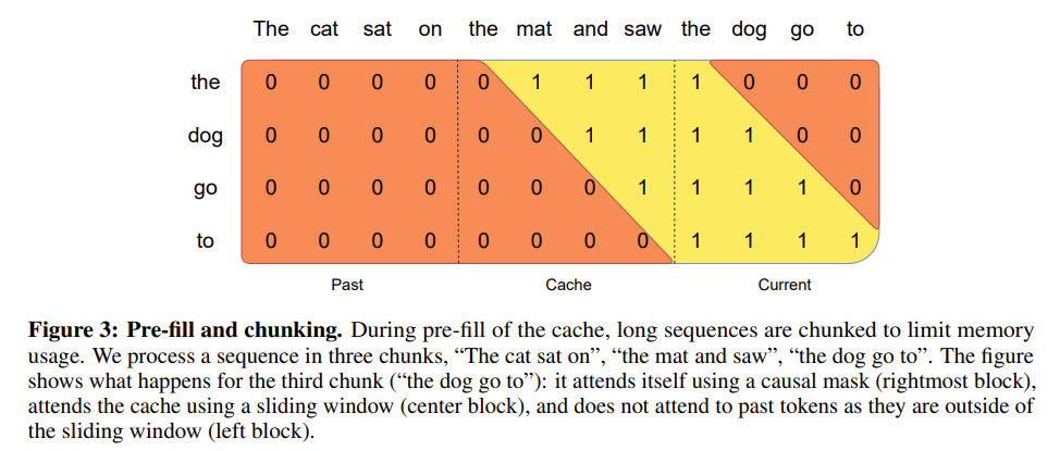
Enhancing Throughput and Efficacy: Cache Strategies

In its pursuit of heightened throughput and effectiveness, Mistral employs two primary strategies concerning its cache: the Rolling Buffer Cache and Pre-filling and Chunking. With a fixed-size cache, entries for timestep $i$ are stored at position $i$ mod $W$ , allowing for overwriting of past values when $i$ exceeds $W$ . This clever use of a rolling buffer curtails cache memory usage without sacrificing model quality. Additionally, by pre-filling the cache with prompt data and processing it in chunks, the model optimizes its performance from the very outset, as illustrated in the figure below.